Simple Regression Worksheet

Directions

Work with one or more other students to complete each of the tasks in this document. As part of this, include the syntax you use to complete each tasks in a script file. As you write your script file, adhere to good coding practices:

• Include comments
• Include spaces
• Include a line break after every pipe operator you use.

You will also need to answer some questions in a Word or Google document.

Task 1: Import Data

Import the riverview.csv data into an object named city. Also, examine the data codebook so you are familiar with the different attributes.

# Load libraries
library(corrr)
library(dplyr)
library(ggplot2)
library(readr)

# Import data
city = read_csv("https://raw.githubusercontent.com/zief0002/modeling/main/data/riverview.csv")

# View data
city

# A tibble: 32 × 5
   education income seniority gender     party      
       <dbl>  <dbl>     <dbl> <chr>      <chr>      
 1         8   26.4         9 female     Independent
 2         8   37.4         7 Not female Democrat   
 3        10   34.2        16 female     Independent
 4        10   25.5         1 female     Republican 
 5        10   47.0        14 Not female Democrat   
 6        12   46.5        11 female     Democrat   
 7        12   52.5        16 female     Independent
 8        12   37.7        14 Not female Democrat   
 9        12   50.3        24 Not female Democrat   
10        14   32.6         5 female     Independent
# ℹ 22 more rows

Task 2: Marginal Distribution of Seniority-level

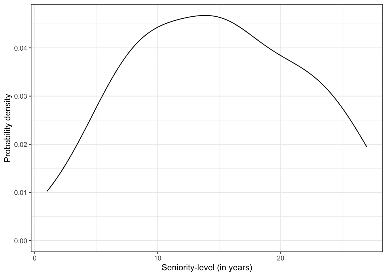
Create a density plot of the years of seniority attribute (seniority). You may also want to produce summary statistics for this attribute. Describe the shape, center (i.e., typical value), and variability. Be sure to use the data context in this description.

# Density plot
ggplot(data = city, aes(x = seniority)) +
  stat_density(geom = "line") +
  theme_bw() +
  xlab("Seniority-level (in years)") +
  ylab("Probability density")

# Summary statistics
city |>
  summarize(
    M = mean(seniority),
    SD = sd(seniority)
    )

# A tibble: 1 × 2
      M    SD
  <dbl> <dbl>
1  14.8  6.95

The marginal distribution of seniority-level is unimodal, and roughly symmetric with a mean of close to 15 years (\(M=14.81\)). There is variation in employees’ seniority-level of education, with most having between 8 and 22 years of seniority (\(SD=6.95\)).

Task 3: Relationship between Seniority-level and Income

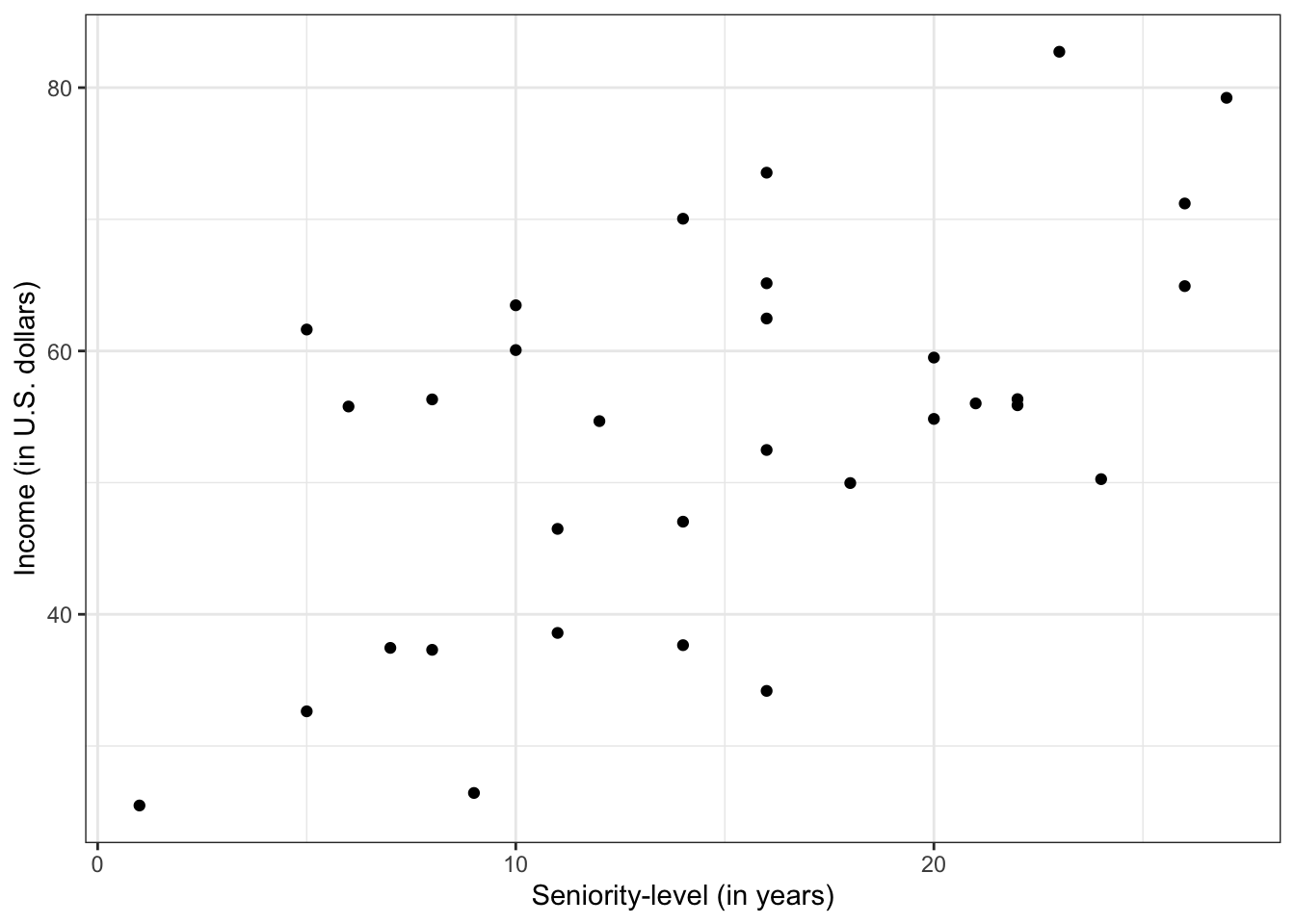
Create a scatterplot of the relationship between seniority-level and income. In this plot assume income is the outcome and seniority-level is the predictor. Describe this relationship by indicating the functional form, direction, magnitude, strength, and any potential outliers. Be sure to use the data context in this description.

ggplot(data = city, aes(x = seniority, y = income)) +
  geom_point() +
  theme_bw() +
  xlab("Seniority-level (in years)") +
  ylab("Income (in U.S. dollars)")

The relationship between seniority-level and income seems linear and positive, suggesting that employees with higher levels of seniority tend to also have higher incomes. The magnitude of this relationship seems somewhat large (steep). The strength of the relationship is weak-to-moderate. There do not appear to be potential outliers in the plot.

Task 4: Compute the Correlation Coefficient

Compute and report the correlation coefficient between seniority-level and income.

city |>
  select(income, seniority) |>
  correlate()

Correlation computed with
• Method: 'pearson'
• Missing treated using: 'pairwise.complete.obs'

# A tibble: 2 × 3
  term      income seniority
  <chr>      <dbl>     <dbl>
1 income    NA         0.582
2 seniority  0.582    NA    

\[ r_{\text{Income, Seniority}} = 0.582 \]

Task 5: Fit the Regression Model

Fit the regression model that uses seniority-level to predict variation in income. Write the fitted equation. Be sure you can write the fitted equation using Equation Editor in Microsoft Word/Google Docs. (This includes adding any hats, or subscripts!)

# Fit regression
lm.1 = lm(income ~ 1 + seniority, data = city)

# View coefficients
lm.1

Call:
lm(formula = income ~ 1 + seniority, data = city)

Coefficients:
(Intercept)    seniority  
     35.690        1.219  

The fitted equation is:

\[ \widehat{\text{Income}_i} = 35.69 + 1.22(\text{Seniority}_i) \]

Task 6: Coefficient Interpretations

Interpret the intercept and slope from the fitted equation.

• Intercept: The predicted mean income for all employees who have 0 years of seniority is 35.69-thousand dollars.
• Slope: Each year of seniority is associated with a 1.22-thousand dollar difference in income, on average.

Task 7: Compute the Sum of Squared Error (SSE) for the Fitted Model

Compute the SSE for the model. Include the syntax you used to compute this.

city |>
  mutate(
    y_hat = 35.69 + 1.22*seniority,
    errors = income - y_hat,
    sq_errors = errors ^ 2
  ) |>
  summarize(
    SSE = sum(sq_errors)
  )

# A tibble: 1 × 1
    SSE
  <dbl>
1 4342.

Task 7: Fit an Intercept-Only Model and Compute the SSE for It

Fit an intercept-only model predicting variation in incomes. Use that model to compute the SSE. Include the syntax you used to compute this.

# Fit intercept-only model (baseline model)
lm.0 = lm(income ~ 1, data = city)

# View coefficients
lm.0

Call:
lm(formula = income ~ 1, data = city)

Coefficients:
(Intercept)  
      53.74  

# Compute SSE for baseline model
city |>
  mutate(
    y_hat = 53.74,
    errors = income - y_hat,
    sq_errors = errors ^ 2
  ) |>
  summarize(
    SSE = sum(sq_errors)
  )

# A tibble: 1 × 1
    SSE
  <dbl>
1 6566.

Task 8: Compute the Proportion Reduction in Error (PRE)

Use the two SSE measures to compute the PRE. Show your work. Also interpret the value using the data’s context.

\[ \begin{split} \text{PRE} &= \frac{6565 - 4342}{6565} \\[2ex] &= \frac{2223}{6565} \\[2ex] &= 0.339 \end{split} \]

33.9% of the variation in employee incomes can be explained by differences in seniority-level.

OR

After including seniority in the model, the amount of unexplained variation in employee incomes was reduced by 33.9%.