📝 Tools for Dealing with Heteroskedasticity

---

In this set of notes, we will use data from Statistics Canada’s Survey of Labour and Income Dynamics (SLID) to explain variation in the hourly wage rate of employed citizens in Ontario.

• [CSV]
• [Codebook]

A script file for the analyses in these notes is also available:

• [R Script File]

Data Exploration

As with any potential regression analysis, we will begin by importing the data and examining the scatterplot of each predictor with the outcome. These plots suggest that each of the predictors is related to the outcome.

# Load libraries
library(broom)
library(car)
library(corrr)
library(ggExtra)
library(patchwork)
library(tidyverse)

# Import data
slid = read_csv("https://raw.githubusercontent.com/zief0002/redesigned-adventure/main/data/slid.csv")

# View data
slid

Note that the read_csv() function can take a URL for a dataset stored on the web.

Here we examine the marginal density plots for the outcome and each continuous predictor, along with the scatterplots showing the relationship between each predictor and the outcome.

Code

d1 = ggplot(data = slid, aes(x = wages)) +
  geom_density() +
  theme_bw() +
  xlab("Hourly wage rate")

d2 = ggplot(data = slid, aes(x = age)) +
  geom_density() +
  theme_bw() +
  xlab("Age (in years)")

d3 = ggplot(data = slid, aes(x = education)) +
  geom_density() +
  theme_bw() +
  xlab("Education (in years)")


p1 = ggplot(data = slid, aes(x = age, y = wages)) +
  geom_point() +
  geom_smooth(method = "lm", se = FALSE) +
  theme_bw() +
  xlab("Age (in years)") +
  ylab("Hourly wage rate")

p2 = ggplot(data = slid, aes(x = age, y = education)) +
  geom_point() +
  geom_smooth(method = "lm", se = FALSE) +
  theme_bw() +
  xlab("Education (in years)") +
  ylab("Hourly wage rate")


p3 = ggplot(data = slid, aes(x = male, y = education)) +
  geom_point() +
  geom_smooth(method = "lm", se = FALSE) +
  theme_bw() +
  xlab("Male") +
  ylab("Hourly wage rate")

(d1 | d2 | d3) / (p1 | p2 | p3)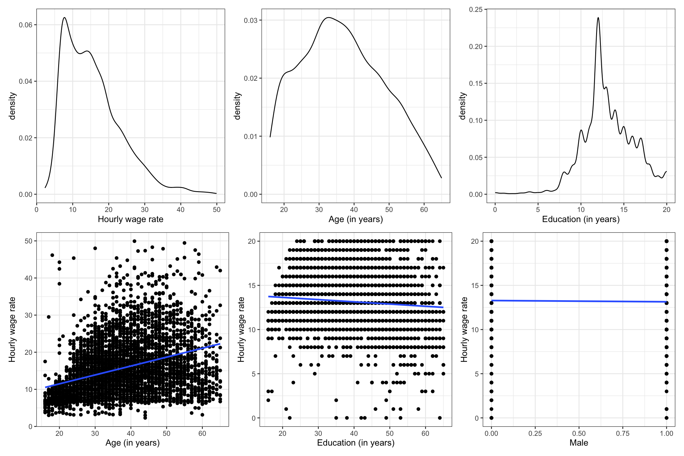

Scatterplot of hourly wage versus each predictor. The fitted regression line is also displayed in each plot.

Based on what we see in these plots, the outcome (hourly wage) looks to be right-skewed. A skewed outcome may or may not be problematic. (It often leads to violations of the conditional normality or homoskedasticity assumption, although we cannot confirm until after we fit the model and examine the residuals.) The relationships between hourly wage and each of the three potential predictors seem linear. The plot with the age predictor, however, foreshadows that we might violate the homoskedasticity assumption (the variance of hourly wages seems to grow for higher ages), but we will withhold judgment until after we fit our multi-predictor model.

Fitting a Multi-Predictor Model

Next, we fit a model regressing wages on the three predictors simultaneously and examine the residual plots. Because we will be looking at residual plots for many different fitted models, we will write and then use a function that creates these plots.

# Function to create residual plots
residual_plots = function(object){
  # Get residuals and fitted values
  aug_lm = broom::augment(object, se_fit = TRUE)

  # Create residual plot
  p1 = ggplot(data = aug_lm, aes(x =.resid)) +
    educate::stat_density_confidence(model = "normal") +
    geom_density() +
    theme_light() +
    xlab("Residuals") +
    ylab("Probability Density")

  # Create residual plot
  p2 = ggplot(data = aug_lm, aes(x =.fitted, y = .resid)) +
    geom_hline(yintercept = 0, linetype = "dashed") +
    geom_point(alpha = 0.1) +
    geom_smooth(method = "lm", se = TRUE) +
    geom_smooth(method = "loess", se = FALSE, n = 50, span = 0.67) +
    theme_light() +
    xlab("Fitted values") +
    ylab("Residuals")


  return(p1 | p2)
}

Note that the {educate} package is not available from CRAN, and only available via GitHub. To install this package use the install_github() function from the {remotes} package to install it. The full syntax is: remotes::install_github("zief0002/educate").

Now we can use our new function to examine the residual plots from the main-effects model.

# Fit model
lm.1 = lm(wages ~ 1 + age + education + male, data = slid)

# Examine residual plots
residual_plots(lm.1)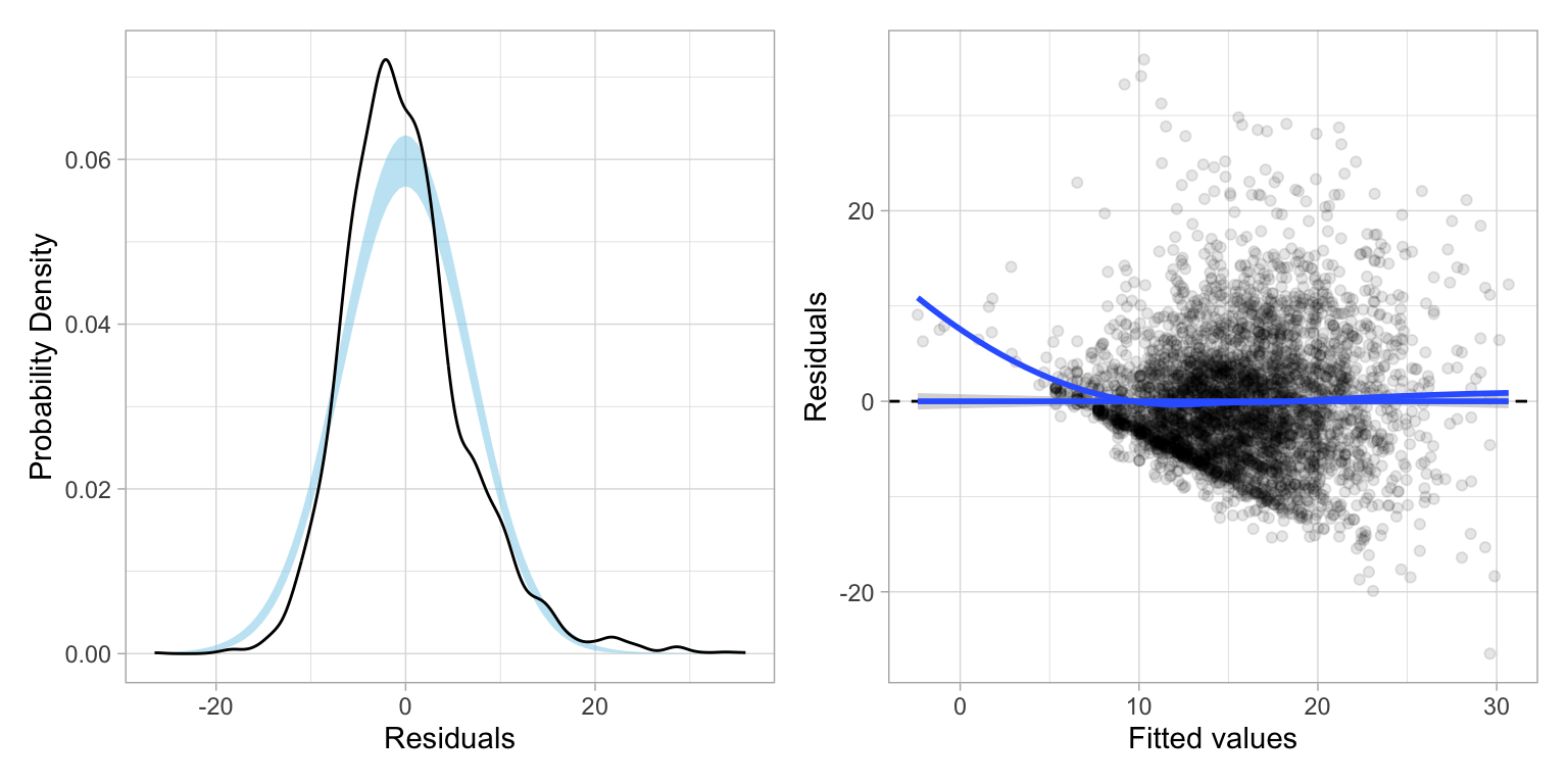

Residual plots for the model that includes the main effects of age, education level, and sex.

Examining the residual plots:

• The linearity assumption may be violated; the loess line suggests some nonlinearity (maybe due to omitted interaction/polynomial terms)
• The normality assumption may be violated; the upper end of the distribution deviates from what would be expected from a normal distribution in the QQ-plot.
• The homoskedasticity assumption is likely violated; the plot of studentized residuals versus the fitted values shows severe fanning; the variation in residuals seems to increase for higher fitted values.

Because of the nonlinearity, we might consider including interaction terms. The most obvious interaction is that between age and education level, as it seems like the effect of age on hourly wage might be moderated by education level. (Remember, do NOT include interactions unless they make theoretical sense!) Below we fit this model, still controlling for sex, and examine the residuals.

# Fit model
lm.2 = lm(wages ~ 1 + age + education + male + age:education, data = slid)

# Examine residual plots
residual_plots(lm.2)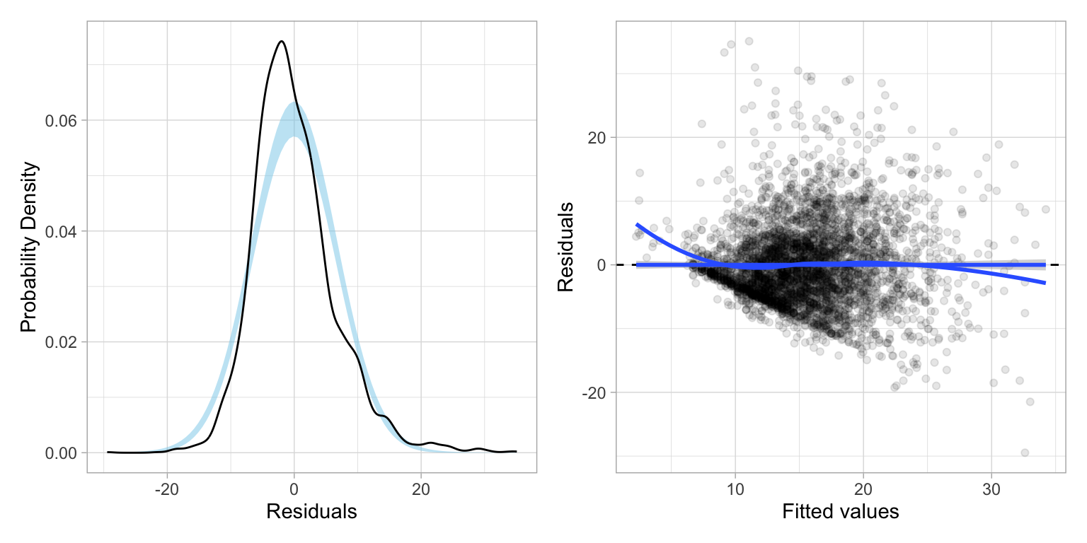

Residual plots for the model that includes an interaction effect between age and education level.

Including the age by education interaction term (age:education) seems to alleviate the nonlinearity issue, but the residual plots indicate there still may be violations of the normality and homoskedasticity assumptions. Violating normality is less problematic here since, given our sample size, the Central Limit Theorem will ensure that the inferences are still approximately valid. Violating homoskedasticity, on the other hand, is more problematic.

Violating Homoskedasticity

Violating the distributional assumption of homoskedasticity results in:

• Incorrect computation of the sampling variances and covariances; and because of this
• The OLS estimates are no longer BLUE (Best Linear Unbiased Estimator).

This means that the SEs (and resulting t- and p-values) for the coefficients are incorrect. In addition, the OLS estimators are no longer the most efficient estimators. How bad this is depends on several factors (e.g., how much the variances differ, sample sizes).

Heteroskedasticity: What is it and How do we Deal with It?

Recall that the variance–covariance matrix for the residuals under the asssumption of homoskedasticity was:

\[ \boldsymbol{\sigma^2}(\boldsymbol{\epsilon}) = \begin{bmatrix}\sigma^2_{\epsilon} & 0 & 0 & \ldots & 0 \\ 0 & \sigma^2_{\epsilon} & 0 & \ldots & 0\\ 0 & 0 & \sigma^2_{\epsilon} & \ldots & 0\\ \vdots & \vdots & \vdots & \ddots & \vdots \\ 0 & 0 & 0 & \ldots & \sigma^2_{\epsilon}\end{bmatrix} \]

Homoskedasticity implies that the variance for each residual was identical, namely \(\sigma^2_{\epsilon}\). Since the variance estimate for each residual was the same, we could estimate a single value for these variances, the residual variance, and use that to obtain the sampling variances and covariances for the coefficients:

\[ \boldsymbol{\sigma^2_B} = \sigma^2_{\epsilon} (\mathbf{X}^{\prime}\mathbf{X})^{-1} \]

Heteroskedasticy implies that the residual variances are not constant. We can represent the variance–covariance matrix of the residuals under heteroskedasticity as:

\[ \boldsymbol{\sigma^2}(\boldsymbol{\epsilon}) = \begin{bmatrix}\sigma^2_{1} & 0 & 0 & \ldots & 0 \\ 0 & \sigma^2_{2} & 0 & \ldots & 0\\ 0 & 0 & \sigma^2_{3} & \ldots & 0\\ \vdots & \vdots & \vdots & \ddots & \vdots \\ 0 & 0 & 0 & \ldots & \sigma^2_{n}\end{bmatrix} \]

In this matrix, each residual has a potentially different variance. Now, there is more than one residual variance, and estimating these variance becomes more complicated, as does estimating the sampling variances and covariances of the regression coefficients.

There are at least three primary methods for dealing with heteroskedasticity: (1) transform the y-values using a variance stabilizing transformation; (2) fit the model using weighted least squares rather than OLS; or (3) adjust the SEs and covariances to account for the non-constant variances. We will examine each of these in turn.

Variance Stabilizing Transformations

The idea behind using a variance stabilizing transformation on the outcome (y) is that the transformed y-values will be homoskedastic. If so, we can fit the OLS regression model using the transformed y-values; the inferences will be valid; and, if necessary, we can back-transform for better interpretations. There are several transformations that can be applied to y that might stabilize the variances. Two common transformations are:

• Log-transformation; \(\ln(Y)_i\)
• Square-root transformation; \(\sqrt{Y_i}\)

Prior to applying these transformations, you may need to add a constant value to each y-value so that all \(y_i>0\) (log-transformation) or all \(y_i \geq 0\) (square-root transformation).

Both of these transformations are power transformations. Power transformations have the mathematical form:

\[ y^*_i = y_i^{p} \]

where \(y^*_i\) is the transformed y-value, \(y_i\) is the original y-value, and p is an integer. The following are all power transformations of y:

\[ \begin{split} & ~\vdots \\[0.5em] & Y^4 \\[0.5em] & Y^3 \\[0.5em] & Y^2 \\[1.5em] & Y^1 = Y \\[1.5em] & Y^{0.5} = \sqrt{Y} \\[0.5em] & Y^0 \equiv \ln(Y) \\[0.5em] & Y^{-1} = \frac{1}{Y} \\[0.5em] & Y^{-2} = \frac{1}{Y^2} \\[0.5em] & ~\vdots \end{split} \]

Powers such that \(p<1\) are referred to as downward transformations, and those with \(p>1\) are referred to as upward transformations. Both the log-transformation and square-root transformation are downward transformations of y. Here we will fit the main effects model using the square-root transformation and the log-transformation of the hourly wage values.

# Create transformed y-values
slid = slid |>
  mutate(
    sqrt_wages = sqrt(wages),
    ln_wages = log(wages)
  )

# Fit models
lm_sqrt = lm(sqrt_wages ~ 1 + age + education + male, data = slid)
lm_ln = lm(ln_wages ~ 1 + age + education + male, data = slid)

The plots below show the residuals based on fitting a model with each of these transformations applied to the wages data.

Code

# Examine residual plots
residual_plots(lm_sqrt) / residual_plots(lm_ln)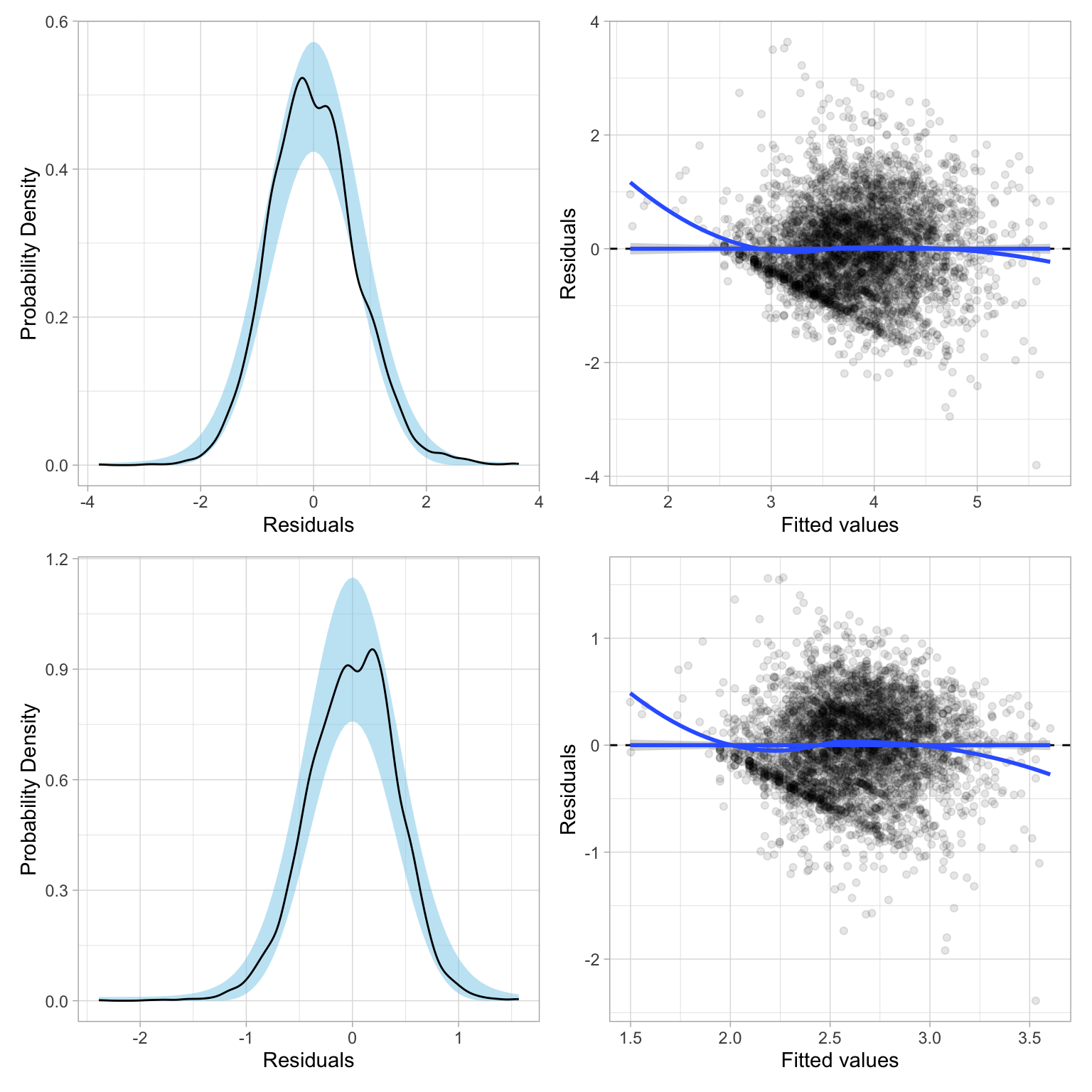

TOP: Residual plots for the main effects model that used a square root transformation on y. BOTTOM: Residual plots for the main effects model that used a logarithmic transformation on y.

Both of these residual plots seem to show less heterogeneity than the residuals from the model with untransformed wages. However, neither transformation, \(p=0\) nor \(p=0.5\), seems to have “fixed” the problem completely.

Box-Cox Transformation

Is there a power transformation that would better “fix” the heteroskedasticity? In their seminal paper, Box & Cox (1964) proposed a series of power transformations that could be applied to data in order to better meet assumptions such as linearity, normality, and homoskedasticity. The general form of the Box-Cox model is:

\[ Y^{(\lambda)}_i = \beta_0 + \beta_1(X1_{i}) + \beta_2(X2_{i}) + \ldots + \beta_k(Xk_{i}) + \epsilon_i \]

where the errors are independent and \(\mathcal{N}(0,\sigma^2_{\epsilon})\), and

\[ Y^{(\lambda)}_i = \begin{cases} \frac{Y_i^{\lambda}-1}{\lambda} & \text{for } \lambda \neq 0 \\[1em] \ln(Y_i) & \text{for } \lambda = 0 \end{cases} \]

This transformation is only defined for positive values of Y.

The powerTransform() function from the {car} library can be used to determine the optimal value of \(\lambda\).

# Find optimal power transformation using Box-Cox
powerTransform(lm.1)

Estimated transformation parameter 
        Y1 
0.08598786 

The output from the powerTransform() function gives the optimal power for the transformation of y, namely \(\lambda = 0.086\). To actually implement the power transformation we use the transform Y based on the Box-Cox algorithm presented earlier.

slid = slid |>
  mutate(
    bc_wages = (wages ^ 0.086 - 1) / 0.086
  )

# Fit models
lm_bc = lm(bc_wages ~ 1 + age + education + male, data = slid)

The residual plots (shown below) indicate better behaved residuals for the main-effects model, although even this optimal transformation still shows some evidence of heteroskedasticity.

Code

# Examine residual plots
residual_plots(lm_bc)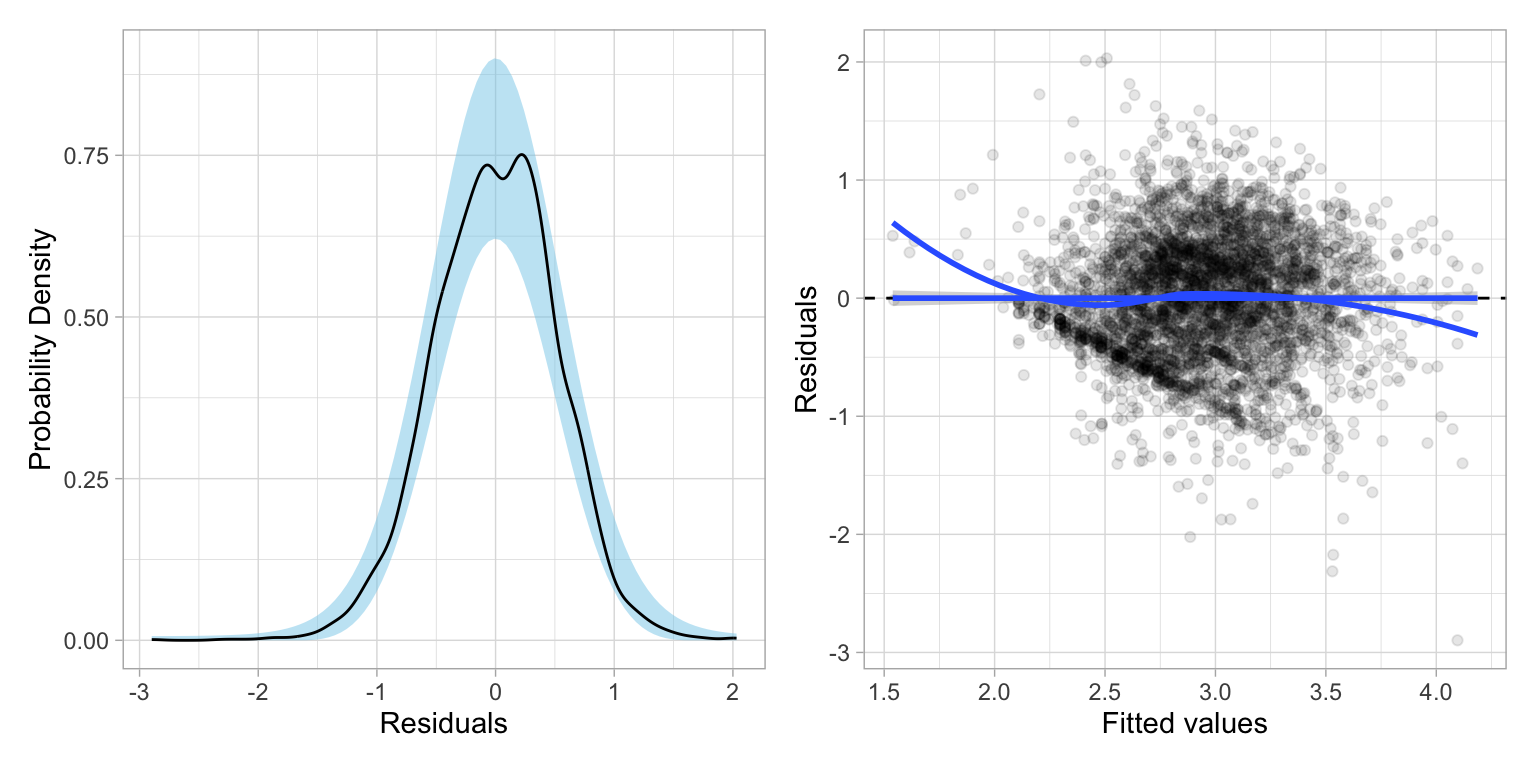

Residual plots for the main effects model that used a Box-Cox transformation on Y with \(\lambda=0.086\).

One problem with using this transformation is that the regression coefficients do not have a direct interpretation. For example, looking at the coefficient-level output:

tidy(lm_bc, conf.int = TRUE)

The age coefficient would be interpreted as: each one-year difference in age is associated with a 0.0227-unit difference in the transformed Y, controlling for differences in education and sex. But what does a 0.227-unit difference in transformed Y mean when we translate that back to wages?

Profile Plot for Different Transformations

Most of the power transformations under Box-Cox would produce coefficients that are difficult to interpret. The exception is when \(\lambda=0\). This is the log-transformation which is directly interpretable. Since the optimal \(\lambda\) value of 0.086 is quite close to 0, we might wonder whether we could just use the log-transformation (\(\lambda=0\)). The Box-Cox algorithm optimizes the log-likelihood of a given model, so the statistical question is whether there is a difference in the log-likelihood produced by the optimal transformation and that for the log-transformation.

To evaluate this, we can plot of the log-likelihood for a given model using a set of lambda values. This is called a profile plot of the log-likelihood. The boxCox() function creates a profile plot of the log-likelihood for a defined sequence of \(\lambda\) values. Here we will plot the profile of the log-likelihood for \(-2 \leq \lambda \leq 2\).

# Plot of the log-likelihood for a given model versus a sequence of lambda values
boxCox(lm.1, lambda = seq(from = -2, to = 2, by = 0.1))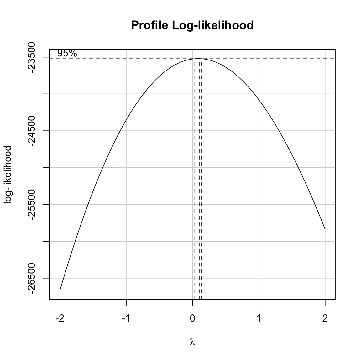

Plot of the log-likelihood profile for a given model versus a sequence of lambda values. The lambda that produces the highest log-likelihood is 0.086, the optimal lambda value.

The profile plot shows that the optimal lambda value, 0.86, produces the maximum log-likelihood value for the given model. We also are shown the 95% confidence limits for lambda based on a test of the curvature of the log-likelihood function. This interval offers a range of \(\lambda\) values that will give comparable transformations. Since the values associated with the confidence limits are not outputted by the boxCox() function, we may need to zoom in to determine these limits by tweaking the sequence of \(\lambda\) values in the boxCox() function.

# Zomm in on confidence limits
boxCox(lm.1, lambda = seq(from = 0.03, to = 0.2, by = .001))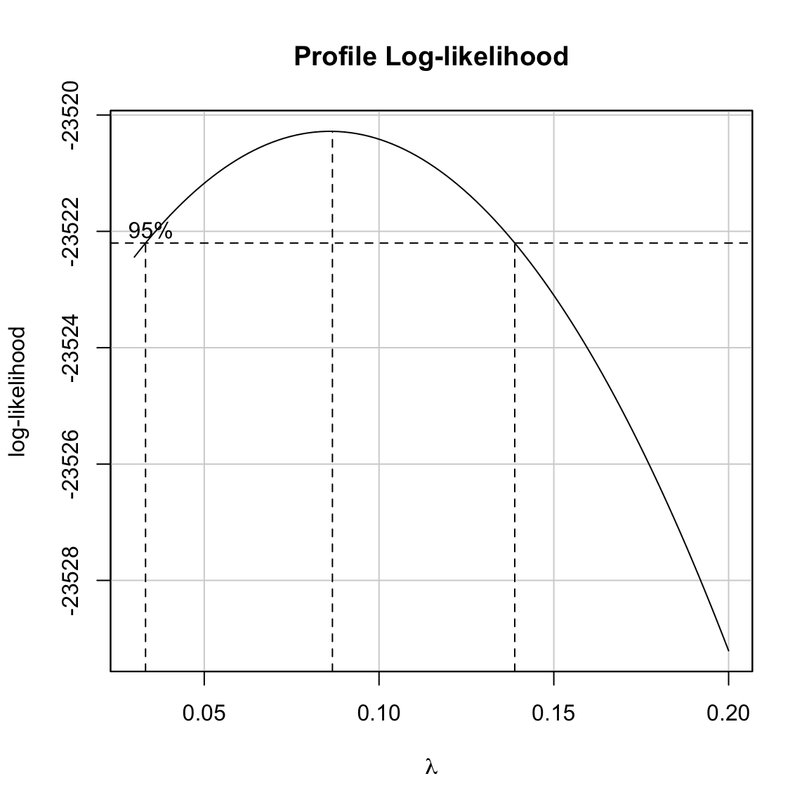

Plot of the log-likelihood profile for a given model versus a narrower sequence of lambda values.

It looks as though \(.03 \leq \lambda \leq 0.14\) all give comparable transformations. Unfortunately, 0 is not included in those limits. This means that the \(\lambda\) value of 0.086 will produce a higher log-likelihood than the log-transformation. It is important to remember that even though the log-likelihood will be optimized, the compatibility with the assumptions may or may not be improved when we use \(\lambda=0.086\) versus \(\lambda=0\). The only way to evaluate this is to fit the models and check the residuals.

Weighted Least Squares Estimation

Another method for dealing with heteroskedasticity is to change the method we use for estimating the coefficients and standard errors. The most common method for doing this is to use weighted least squares (WLS) estimation rather than ordinary least squares (OLS).

Under heteroskedasticity recall that the residual variance of the ith residual is \(\sigma^2_i\), and the variance–covariance matrix of the residuals is defined as,

\[ \boldsymbol{\Sigma} = \begin{bmatrix}\sigma^2_{1} & 0 & 0 & \ldots & 0 \\ 0 & \sigma^2_{2} & 0 & \ldots & 0\\ 0 & 0 & \sigma^2_{3} & \ldots & 0\\ \vdots & \vdots & \vdots & \ddots & \vdots \\ 0 & 0 & 0 & \ldots & \sigma^2_{n}\end{bmatrix}, \]

This implies that the n observations no longer have the same reliability (i.e., precision of estimation). Observations with small variances have more reliability than observations with large variances. The idea behind WLS estimation is that those observations that are less reliable are down-weighted in the estimation of the overall error variance.

Assume Error Variances are Known

Let’s assume that each of the error variances, \(\sigma^2_i\), are known. This is generally not a valid assumption, but it gives us a point to start from. If we know these values, we can modify the likelihood function from OLS by substituting these values in for the OLS error variance, \(\sigma^2_{\epsilon}\).

\[ \begin{split} \mathrm{OLS:} \qquad \mathcal{L}(\boldsymbol{\beta}) &= \prod_{i=1}^n \frac{1}{\sqrt{2\pi\sigma^2_{\epsilon}}}\exp\left[-\frac{1}{2\sigma^2_{\epsilon}} \big(Y_i-\beta_0 - \beta_1X_{1i} - \beta_2X_{2i} - \ldots - \beta_kX_{ki}\big)^2\right] \\[1em] \mathrm{WLS:} \qquad \mathcal{L}(\boldsymbol{\beta}) &= \prod_{i=1}^n \frac{1}{\sqrt{2\pi\sigma^2_{i}}}\exp\left[-\frac{1}{2\sigma^2_{i}} \big(Y_i-\beta_0 - \beta_1X_{1i} - \beta_2X_{2i} - \ldots - \beta_kX_{ki}\big)^2\right] \end{split} \]

Next, we define the reciprocal of the error variances as \(w_i\), or weight:

\[ w_i = \frac{1}{\sigma^2_i} \]

This can be used to simplify the likelihood function for WLS:

\[ \begin{split} \mathcal{L}(\boldsymbol{\beta}) &= \bigg[\prod_{i=1}^n \sqrt{\frac{w_i}{2\pi}}\bigg]\exp\left[-\frac{1}{2} \sum_{i=1}^n w_i\big(Y_i-\beta_0 - \beta_1X_{1i} - \beta_2X_{2i} - \ldots - \beta_kX_{ki}\big)^2\right] \end{split} \]

We can then find the coefficient estimates by maximizing \(\mathcal{L}(\boldsymbol{\beta})\) with respect to each of the coefficients; these derivatives will result in k normal equations. Solving this system of normal equations we find that:

\[ \mathbf{b}_{\mathrm{WLS}} = (\mathbf{X}^{\intercal}\mathbf{W}\mathbf{X})^{-1}\mathbf{X}^{\intercal}\mathbf{W}\mathbf{y} \]

where W is a diagonal matrix of the weights,

\[ \mathbf{W} = \begin{bmatrix}w_{1} & 0 & 0 & \ldots & 0 \\ 0 & w_{2} & 0 & \ldots & 0\\ 0 & 0 & w_{3} & \ldots & 0\\ \vdots & \vdots & \vdots & \ddots & \vdots \\ 0 & 0 & 0 & \ldots & w_{n}\end{bmatrix} \]

The variance–covariance matrix for the regression coefficients can then be computed using:

\[ \boldsymbol{\sigma^2}(\mathbf{B}) = \sigma^2_{\epsilon}(\mathbf{X}^{\intercal}\mathbf{W}\mathbf{X})^{-1} \]

where the estimate for \(\sigma^2_{\epsilon}\) is based on a weighted sum of squares:

\[ \hat\sigma^2_{\epsilon} = \frac{\sum_{i=1}^n w_i \times \epsilon_i^2}{n - k - 1} \]

Which can be expressed in matrix algebra as a function of the weight matrix and residual vector as:

\[ \hat\sigma^2_{\epsilon} = \frac{(\mathbf{We})^{\intercal}\mathbf{e}}{n - k - 1} \]

An Example of WLS Estimation

To illustrate WLS, consider the following data which includes average ACT scores for a classroom of students, ACT score for the teacher, and the standard deviation of the class ACT scores.

Class Average ACT	Teacher ACT	Class SD
17.3	21	5.99
17.1	20	3.94
16.4	19	1.90
16.4	18	0.40
16.1	17	5.65
16.2	16	2.59

Suppose we want to use the teacher’s ACT score to predict variation in the class average ACT score. Fitting this model using OLS, we can compute the coefficient estimates and the standard errors for each coefficient.

# Enter y vector
y = c(17.3, 17.1, 16.4, 16.4, 16.1, 16.2)

# Create design matrix
X = matrix(
  data = c(rep(1, 6), 21, 20 , 19, 18, 17, 16),
  ncol = 2
)

# Compute coefficients
b = solve(t(X) %*% X) %*% t(X) %*% y

# Compute SEs for coefficients
e = y - X %*% b
sigma2_e = t(e) %*% e / (6 - 1 - 1)
V_b = as.numeric(sigma2_e) * solve(t(X) %*% X)
sqrt(diag(V_b))

[1] 0.98356794 0.05294073

We could also have used built-in R functions to obtain these values:

lm.ols = lm(y ~ 1 + X[ , 2])
tidy(lm.ols, conf.int = TRUE)

The problem, of course, is that the variation in the residuals is not constant as the reliability for the 10 class average ACT values is not the same for each class; the standard deviations are different. Because of this, we may want to fit a WLS regression model rather than an OLS model.

# Set up weight matrix, W
class_sd = c(5.99, 3.94, 1.90, 0.40, 5.65, 2.59)
w_i = 1 / (class_sd ^ 2)
W = diag(w_i)
W

          [,1]       [,2]      [,3] [,4]       [,5]      [,6]
[1,] 0.0278706 0.00000000 0.0000000 0.00 0.00000000 0.0000000
[2,] 0.0000000 0.06441805 0.0000000 0.00 0.00000000 0.0000000
[3,] 0.0000000 0.00000000 0.2770083 0.00 0.00000000 0.0000000
[4,] 0.0000000 0.00000000 0.0000000 6.25 0.00000000 0.0000000
[5,] 0.0000000 0.00000000 0.0000000 0.00 0.03132587 0.0000000
[6,] 0.0000000 0.00000000 0.0000000 0.00 0.00000000 0.1490735

# Compute coefficients
b_wls = solve(t(X) %*% W %*% X) %*% t(X) %*% W %*% y
b_wls

           [,1]
[1,] 13.4154764
[2,]  0.1658431

# Compute standard errors for coefficients
e_wls = y - X %*% b_wls                                 # Compute errors from WLS
mse_wls = (t(W %*% e_wls) %*% e_wls) / (6 - 1 - 1)      # Compute MSE estimate
v_b_wls = as.numeric(mse_wls) * solve(t(X) %*% W %*% X) # Compute variance-covariance matrix for B
sqrt(diag(v_b_wls))

[1] 1.17680463 0.06527187

The results of fitting both the OLS and WLS models appear below. Comparing the two sets of results, there is a difference in the coefficient values and in the estimated SEs when using WLS estimation rather than OLS estimation. This would also impact any statistical inference as well.

	OLS		WLS
Coefficient	B	SE	B	SE
Intercept	12.0905	0.9836	13.4155	1.1768
Effect of Teacher ACT Score	0.2429	0.0529	0.1658	0.0653

Fitting the WLS estimation in the lm() Function

The lm() function can also be used to fit a model using WLS estimation. To do this we include the weights= argument in lm(). This takes a vector of weights representing the \(w_i\) values for each of the n observations.

# Create weights vector
w_i = 1 / (class_sd ^ 2)

# Fit WLS model
lm_wls = lm(y ~ 1 + X[ , 2], weights = w_i)
tidy(lm_wls, conf.int = TRUE)

Not only can we use tidy() and glance() to obtain coefficient and model-level summaries, but we can also use augment(), anova(), or any other function that takes a fitted model as its input.

What if Error Variances are Unknown?

The previous example assumed that the variance–covariance matrix of the residuals was known. In practice, this is almost never the case. When we do not know the error variances, we need to estimate them from the data.

One method for estimating the error variances for each observation, is:

1. Fit an OLS model to the data, and obtain the residuals.
2. Square these residuals and regress them (using OLS) on the same set of predictors.
3. Obtain the fitted values from Step 2.
4. Create the weights using \(w_i = \frac{1}{\hat{y}_i}\) where \(\hat{y}_i\) are the fitted values from Step 3.
5. Fit the WLS using the weights from Step 4.

This is a two-stage process in which we (1) estimate the weights, and (2) use those weights in the WLS estimation. We will illustrate this methodology using the SLID data.

# Step 1: Fit the OLS regression
lm_step_1 = lm(wages ~ 1 + age + education + male + age:education, data = slid)

# Step 2: Obtain the residuals and square them
out_1 = augment(lm_step_1) |>
  mutate(
    e_sq = .resid ^ 2
  )

# Step 2: Regresss e^2 on the predictors from Step 1
lm_step_2 = lm(e_sq ~ 1 + age + education + male + age:education, data = out_1)

# Step 3: Obtain the fitted values from Step 2
y_hat = fitted(lm_step_2)


# Step 4: Create the weights
w_i = 1 / (y_hat ^ 2)

# Step 5: Use the fitted values as weights in the WLS
lm_step_5 = lm(wages ~ 1 + age + education + male + age:education, data = slid, weights = w_i)

Before examining any output from this model, let’s examine the residual plots. The residual plots suggest that the homoskedasticity assumption is much more reasonably satisfied after using WLS estimation; although it is still not perfect. The normality assumption looks untenable here.

One way to proceed would be to apply a variance stabilizing transformation to y (e.g., log-transform) and then fit a WLS model. To do this you would go through the steps of estimating the weights again based on the transformed y.

Code

# Examine residual plots
residual_plots(lm_step_5)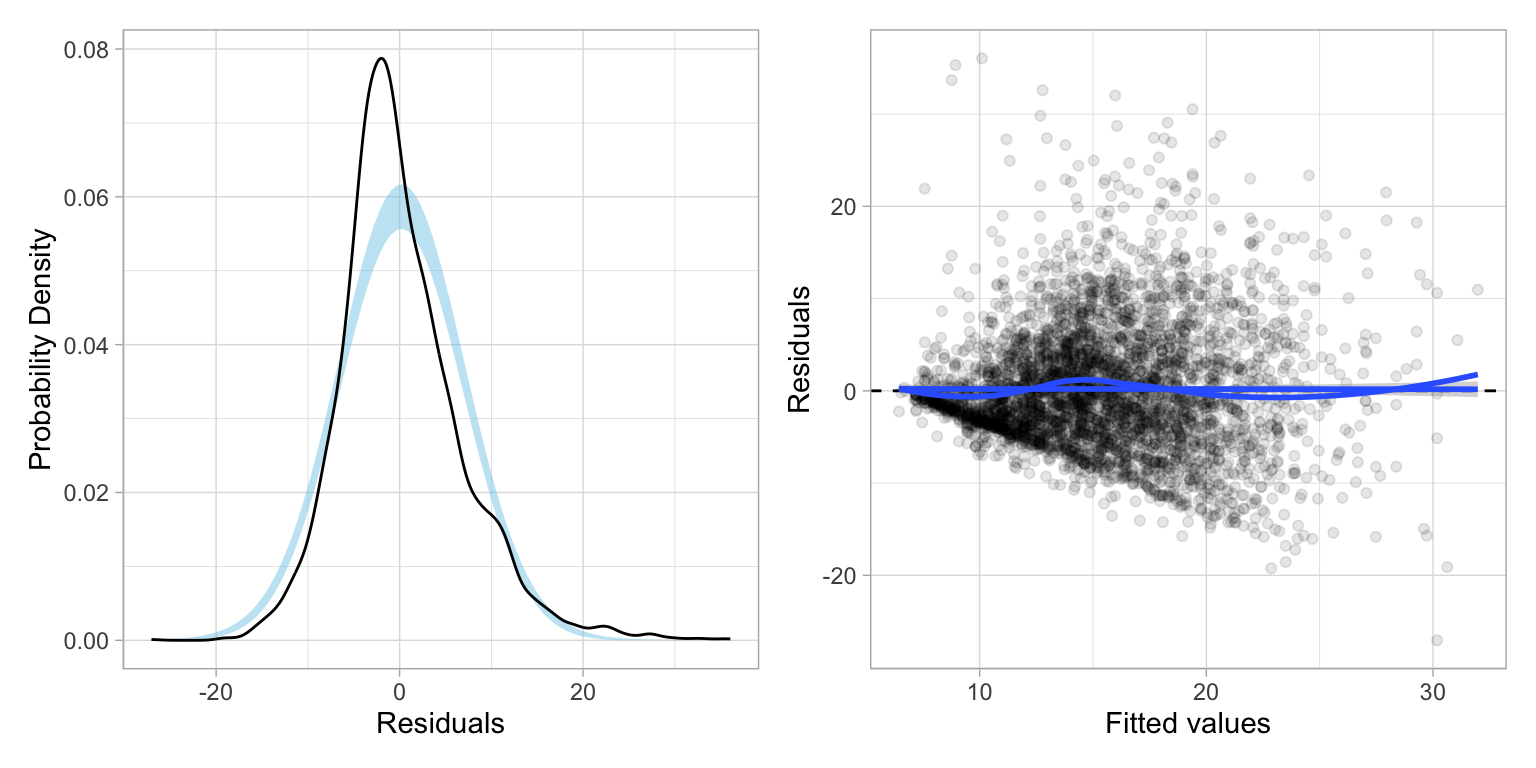

Residual plots for the model that includes the main effects of age, education level, and sex fitted with WLS estimation.

The WLS coefficient estimates, standard errors, and coefficient-level inference are presented below.

# Examine coefficient-level output
tidy(lm_step_5, conf.int = TRUE)

Adjusting the Standard Errors: Sandwich Estimation

Since the primary effect of heteroskedasticity is that the sampling variances and covariances are incorrect, one method of dealing with this assumption violation is to use the OLS coefficients (which are still unbiased under heteroskedasticity), but make adjustments to the variance–covariance matrix of the coefficients. We can compute the adjusted variance–covariance matrix of the regression coefficients using:

\[ V(\mathbf{b}) = (\mathbf{X}^{\intercal}\mathbf{X})^{-1}\mathbf{X}^{\intercal}\boldsymbol{\Sigma}\mathbf{X} (\mathbf{X}^{\intercal}\mathbf{X})^{-1} \]

where, \(\boldsymbol{\Sigma}\) is the variance-covariance matrix of the residuals.

This is often referred to as a sandwich estimator because the \(\mathbf{X}^{\intercal}\boldsymbol{\Sigma}\mathbf{X}\) is “sandwiched” between two occurrences of \((\mathbf{X}^{\intercal}\mathbf{X})^{-1}\).

Note that under the standard regression assumptions (including homoskedasticity), \(\boldsymbol{\Sigma} = \sigma^2_{\epsilon}\mathbf{I}\), and this whole expression can be simplified to the matrix expression of the variance–covariance matrix for the coefficients under the OLS model.:

\[ \begin{split} V(\mathbf{b}) &= (\mathbf{X}^{\intercal}\mathbf{X})^{-1}\mathbf{X}^{\intercal}\sigma^2_{\epsilon}\mathbf{IX} (\mathbf{X}^{\intercal}\mathbf{X})^{-1} \\[2ex] &= \sigma^2_{\epsilon}(\mathbf{X}^{\intercal}\mathbf{X})^{-1}\mathbf{X}^{\intercal}\mathbf{IX} (\mathbf{X}^{\intercal}\mathbf{X})^{-1} \\[2ex] &= \sigma^2_{\epsilon}(\mathbf{X}^{\intercal}\mathbf{X})^{-1}\mathbf{X}^{\intercal}\mathbf{X} (\mathbf{X}^{\intercal}\mathbf{X})^{-1} \\[2ex] &= \sigma^2_{\epsilon} \mathbf{I} (\mathbf{X}^{\intercal}\mathbf{X})^{-1} \\[2ex] &= \sigma^2_{\epsilon} (\mathbf{X}^{\intercal}\mathbf{X})^{-1} \end{split} \]

If the errors are, however, heteroskedastic, then we need to use the heteroskedastic variance–covariance of the residuals,

\[ \boldsymbol{\Sigma} = \begin{bmatrix}\sigma^2_{1} & 0 & 0 & \ldots & 0 \\ 0 & \sigma^2_{2} & 0 & \ldots & 0\\ 0 & 0 & \sigma^2_{3} & \ldots & 0\\ \vdots & \vdots & \vdots & \ddots & \vdots \\ 0 & 0 & 0 & \ldots & \sigma^2_{n}\end{bmatrix}, \]

One of the computational formulas for variance of a random variable X, using the rules of expectation is:

\[ \sigma^2_X = \mathbb{E}\bigg(\big[X_i - \mathbb{E}(X)\big]^2\bigg) \]

This means for the ith error variance, \(\sigma^2_i\), can be computed as

\[ \sigma^2_{i} = \mathbb{E}\bigg(\big[\epsilon_i - \mathbb{E}(\epsilon)\big]^2\bigg) \]

Which, since \(\mathbb{E}(\epsilon)=0\) simplifies to

\[ \sigma^2_{i} = \mathbb{E}\big(\epsilon_i^2\big) \]

This suggests that we can estimate \(\boldsymbol{\Sigma}\) as:

\[ \hat{\boldsymbol{\Sigma}} = \begin{bmatrix}\epsilon^2_{1} & 0 & 0 & \ldots & 0 \\ 0 & \epsilon^2_{2} & 0 & \ldots & 0\\ 0 & 0 & \epsilon^2_{3} & \ldots & 0\\ \vdots & \vdots & \vdots & \ddots & \vdots \\ 0 & 0 & 0 & \ldots & \epsilon^2_{n}\end{bmatrix}, \]

In other words, the estimated variance–covariance matrix of the residuals under heteroskedasticity is a diagonal matrix with elements that are the squared residuals from the OLS model.

Going back to our SLID example, we can compute the adjusted variance–covariance matrix of the coefficients by using the sandwich estimation method.

# Fit OLS model
lm.ols = lm(wages ~ 1 + age + education + male, data = slid)

# Design matrix
X = model.matrix(lm.1)

# Create Sigma matrix
e_squared = augment(lm.1)$.resid ^ 2
Sigma = e_squared * diag(3997)

# Variance-covariance matrix for B
V_b_adj = solve(t(X) %*% X) %*% t(X) %*% Sigma %*% X %*% solve(t(X) %*% X)

# Compute SEs
sqrt(diag(V_b_adj))

(Intercept)         age   education        male 
0.635836527 0.008807793 0.038468695 0.207141705 

The SEs we produce from this method are typically referred to as Huber-White standard errors because they were introduced in a paper by Huber (1967) and their some of their statistical properties were proved in a paper by White (1980).

Modifying the Huber-White Estimates

Simulation studies by Long & Ervin (2000) suggest a slight modification to the Huber-White estimates; by using a slightly different \(\boldsymbol\Sigma\) matrix:

\[ \hat{\boldsymbol{\Sigma}} = \begin{bmatrix}\frac{\epsilon^2_{1}}{(1-h_{11})^2} & 0 & 0 & \ldots & 0 \\ 0 & \frac{\epsilon^2_{2}}{(1-h_{22})^2} & 0 & \ldots & 0\\ 0 & 0 & \frac{\epsilon^2_{3}}{(1-h_{33})^2} & \ldots & 0\\ \vdots & \vdots & \vdots & \ddots & \vdots \\ 0 & 0 & 0 & \ldots & \frac{\epsilon^2_{n}}{(1-h_{nn})^2}\end{bmatrix}, \]

where, \(h_{ii}\) is the ith diagonal element from the H matrix.

We can compute this modification by adjusting the e_squared value in the R syntax as:

# Sigma matrix
e_squared = augment(lm.1)$.resid ^ 2  / ((1 - augment(lm.1)$.hat) ^ 2)
Sigma = e_squared * diag(3997)

# Variance-covariance matrix for B
V_b_hw_mod = solve(t(X) %*% X) %*% t(X) %*% Sigma %*% X %*% solve(t(X) %*% X)

# Compute adjusted SEs
sqrt(diag(V_b_hw_mod))

(Intercept)         age   education        male 
0.637012622 0.008821005 0.038539628 0.207364732 

We could use these SEs to compute the t-values, associated p-values, and confidence intervals for each of the coefficients.

The three sets of SEs are:

	SE
Coefficient	OLS	Huber-White	Modified Huber-White
Intercept	0.5989773	0.6358365	0.6370126
Age	0.0086640	0.0088078	0.0088210
Education	0.0342567	0.0384687	0.0385396
Age x Education	0.2070092	0.2071417	0.2073647

In these data, the modified Huber-White adjusted SEs are quite similar to the SEs we obtained from OLS, despite the heteroskedasticity observed in the residuals. One advantage of this method is that we do not have to have a preconceived notion of the underlying pattern of variation like we do to use WLS estimation. (We can estimate the pattern using the multi-step approach introduced earlier, but this assumes that the method of estimation correctly mimics the pattern of variation.) If, however, we can identify the pattern of variation, then WLS estimation will produce more efficient (smaller) standard errors than sandwich estimation.

References

Box, G. E. P., & Cox, D. R. (1964). An analysis of transformations. Journal of the Royal Statisistical Society, Series B, 26, 211–246.

Huber, P. J. (1967). The behavior of maximum likelihood estimates under nonstandard conditiona. In L. M. Le Cam & J. Neyman (Eds.), Proceedings of the fifth berkeley symposium on mathematical statistics and probability (pp. 221–233). Berkeley, CA: University of California Press.

Long, J. S., & Ervin, L. H. (2000). Using heteroskedasticity consistent standard errors in the linear regression model. The American Statistician, 54, 217–224.

White, H. (1980). A heteroskedasticity-consistent covariance matrix estimator and a direct test for heteroskedasticity. Econometrica, 38, 817–838.