my_t <- t_test(
  ~Taps | Group, data = caff,
  alternative = "two.sided",
  var.equal = TRUE
) Day 14
Hypothesis Testing for Comparing Two Means
EPSY 5261 : Introductory Statistical Methods
Learning Goals
At the end of this lesson, you should be able to …
- Describe the purpose of a hypothesis test for comparing groups.
- List the steps of a hypothesis test.
- Describe a parametric approach to hypothesis testing for comparing two means.
- List the assumptions for using the t-distribution to test for a difference in means.
- Conceptually understand Type I and Type II errors.
Recall: Attribute Types
- When working with quantitative data, the population mean (\(\mu\)) has been our parameter of interest.
- Sometimes we have two groups (categorical variable) that we want to compare a quantitative outcome on.
- The parameter of interest is now \(\mu_{\text{Group 1}}-\mu_{\text{Group 2}}\).
Purpose of Hypothesis Testing
To test a claim about a population parameter
- One Group
- RQ: Did the average movie length increase in 2022?
- Two Groups
- RQ: Is there a difference in average movie length between dramas and comedies?
Steps of Hypothesis Testing
- Formulate a research question
- Write your hypotheses
- Find sampling distribution assuming the null hypothesis is true
- Compare sample summary to the distribution under the null hypothesis
- Get a p-value
- Make a decision based on the p-value
- Communicate your conclusion in context
Theoretical Distribution
- t-distribution
- Same as for a single mean
- This time we will compare the sample difference in means to the t-distribution
Assumptions
- The distribution of values in both populations are normally distributed.
- Note: If the sample size is greater than 30 in each group we can use the t-distribution without our sample being normally distributed (because of the Central Limit Theorem)
- The values in both populations are independent from each other. (This is the case if we have a random sample.)
- Both populations have the same variance. (This is okay if the larger sample variance not 4x larger than the smaller sample variance):
\[ \frac{\text{Larger } SD^2}{\text{Smaller } SD^2} < 4 \]
Research Question
Is there a difference in the average number of times someone will tap their finger in a minute between those that have had caffeine and those that haven’t had caffeine?
Data
| Group | Taps |
|---|---|
| Caffeine | 230 |
| No Caffeine | 235 |
| Caffeine | 258 |
| ⋮ | ⋮ |
Statistical Hypotheses
- Null hypothesis: There is no difference in the average number of times someone will tap their finger in a minute between those that have had caffeine and those that haven’t had caffeine.
- Alternative hypothesis: There is a difference in the average number of times someone will tap their finger in a minute between those that have had caffeine and those that haven’t had caffeine.
\[ {\begin{split} H_0: \mu_{\text{Caffeine}} &= \mu_{\text{No Caffeine}}\\ H_A: \mu_{\text{Caffeine}} &\neq \mu_{\text{No Caffeine}} \end{split} } \quad \text{OR} \quad {\begin{split} H_0: \mu_{\text{Caffeine}} - \mu_{\text{No Caffeine}} &= 0\\ H_A: \mu_{\text{Caffeine}} - \mu_{\text{No Caffeine}} &\neq 0 \end{split} } \]
Sample Mean Difference
- We will compare our sample mean difference to a t-distribution
- We will compute the mean for each group
- Then we will subtract the mean for the no caffeine group from the mean for the caffeine group
- The order you subtract matters when working in R Studio. R Studio will recognize the first group as the first name alphabetically. So you want to subtract in that same order. (e.g., “Caffeine” is alphabetically before “No caffeine”, so it will compute the difference as “Caffeine” \(-\) “No caffeine”.)
- Mean Taps for Caffeine: 248.3
- Mean Taps for No Caffeine: 244.8
- Sample mean difference: \(248.3 - 244.8 = 3.5\)
R Studio
Compare Sample Difference to Null Distribution
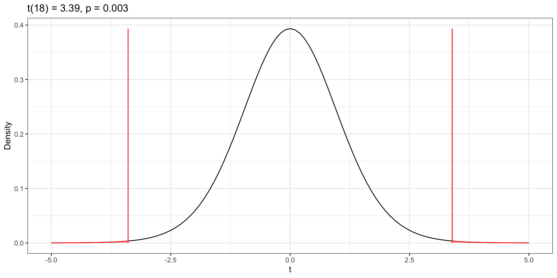
p-Value and Decision
Conclusion
We can conclude that it is likely there is a difference in the average number of finger taps someone will do if they have had caffeine compared to those that have not.
Type I and Type II Errors
Errors in Hypothesis Testing
- When we conduct a hypothesis test, we come to a conclusion based on a p-value…
- Reject the null hypothesis OR fail to reject the null hypothesis
- However, this conclusion could be “incorrect”
- There are two ways to come to an incorrect conclusion depending on our p-value:
- We got a low p-value and rejected the null hypothesis, but we should not have based on the true population parameter.
- We got a high p-value and failed to reject the null hypothesis, but we should have based on the true population parameter
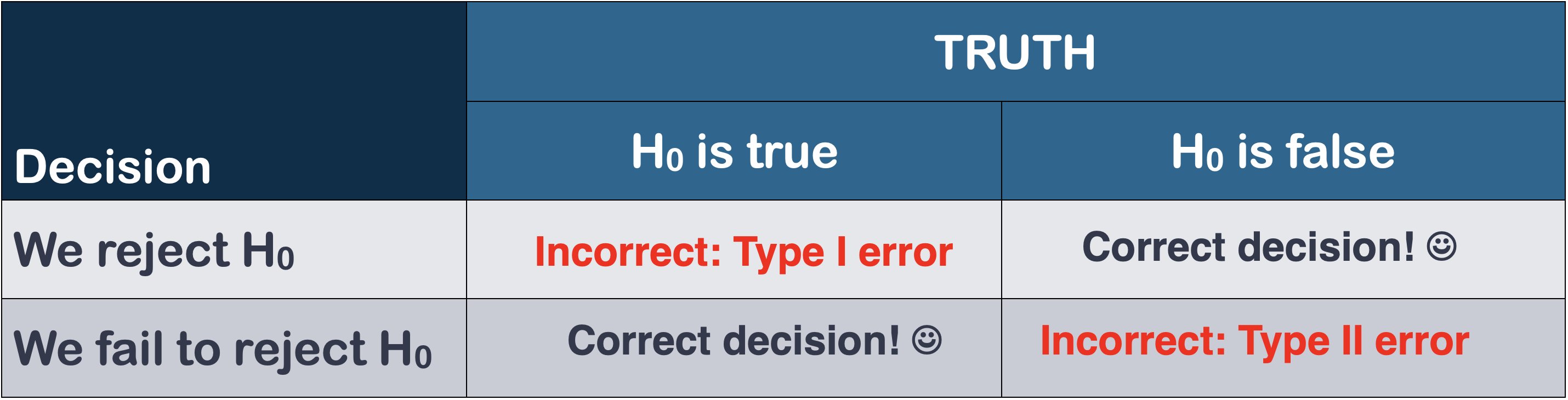
Errors in Hypothesis Testing (cntd.)
- Type I error: We say there is a significant result, when there really is NOT.
- Type II error: We say there is NOT a significant result, when there really IS.
Example: Drug Trial
Consider a drug trial with the following statistical hypotheses:
\[ \begin{split} H_0:& \text{Drug does not work better than placebo} \\ H_A:& \text{Drug works better than placebo} \end{split} \]
Example: Type I Error
Based on a small p-value:
- Decision: We rejected the null hypothesis
We could have made a Type I error. Based on the results of the hypothesis test we concluded that there is a difference; that the drug works better than the placebo. But, in reality there is no difference—the drug actually doesn’t work better than the placebo.
- Consequence: A not useful drug gets sold on the market
Example: Type II Error
Based on a large p-value:
- Decision: We failed to reject the null hypothesis
We could have made a Type II error. Based on the results of the hypothesis test we concluded that there is no difference; that the drug does not work better than the placebo. But, in reality there is a difference—the drug actually does work better than the placebo.
- Consequence: Potentially beneficial drug does not get sold!
Use R Studio
- Use the t-distribution to help us get our estimate for the variability
- Use functions in R Studio to also give us our p-value
- Explore the entire hypothesis test process and consider type I and type II errors in today’s activity
Hypothesis Testing for Comparing Two Means Activity
Summary
- Hypothesis tests help us test a claim while taking into account sampling variability.
- They provide one form of evidence to help answer a research question.
- We can use a t-distribution to help us conduct our test when we have two groups to compare on a quantitative attribute.
- Though we have done our data collection and test with care, we still could have made an error in our conclusion.