Day 24
Introduction to Linear Regression


EPSY 5261 : Introductory Statistical Methods

Learning Goals

At the end of this lesson, you should be able to …

  • Explain when to use linear regression.
  • Write a linear regression equation.
  • Interpret the coefficients in a linear regression equation.
  • Calculate and interpret a residual.
  • Interpret an \(R^2\) value.

If we have a linear relationship we might consider doing a linear regression.

Regression Line

  • “Best fitting” line that describes the relationship between X and Y
  • “Best fit” = Line found by minimizing the squared vertical distances between the points and the line (least squares)

Linear Regression Equation

  • Remember equation for a line from high school math class: \(y = mx + b\).

\[ \hat{y} = \underbrace{\beta_0}_{\text{Intercept}} + \underbrace{\beta_1}_{\text{Slope}}(x) \]

Example

\[ \widehat{\text{Coffees}} = 491 - 5.3(\text{Temperature}) \]

Using R Studio

# Fit regression model
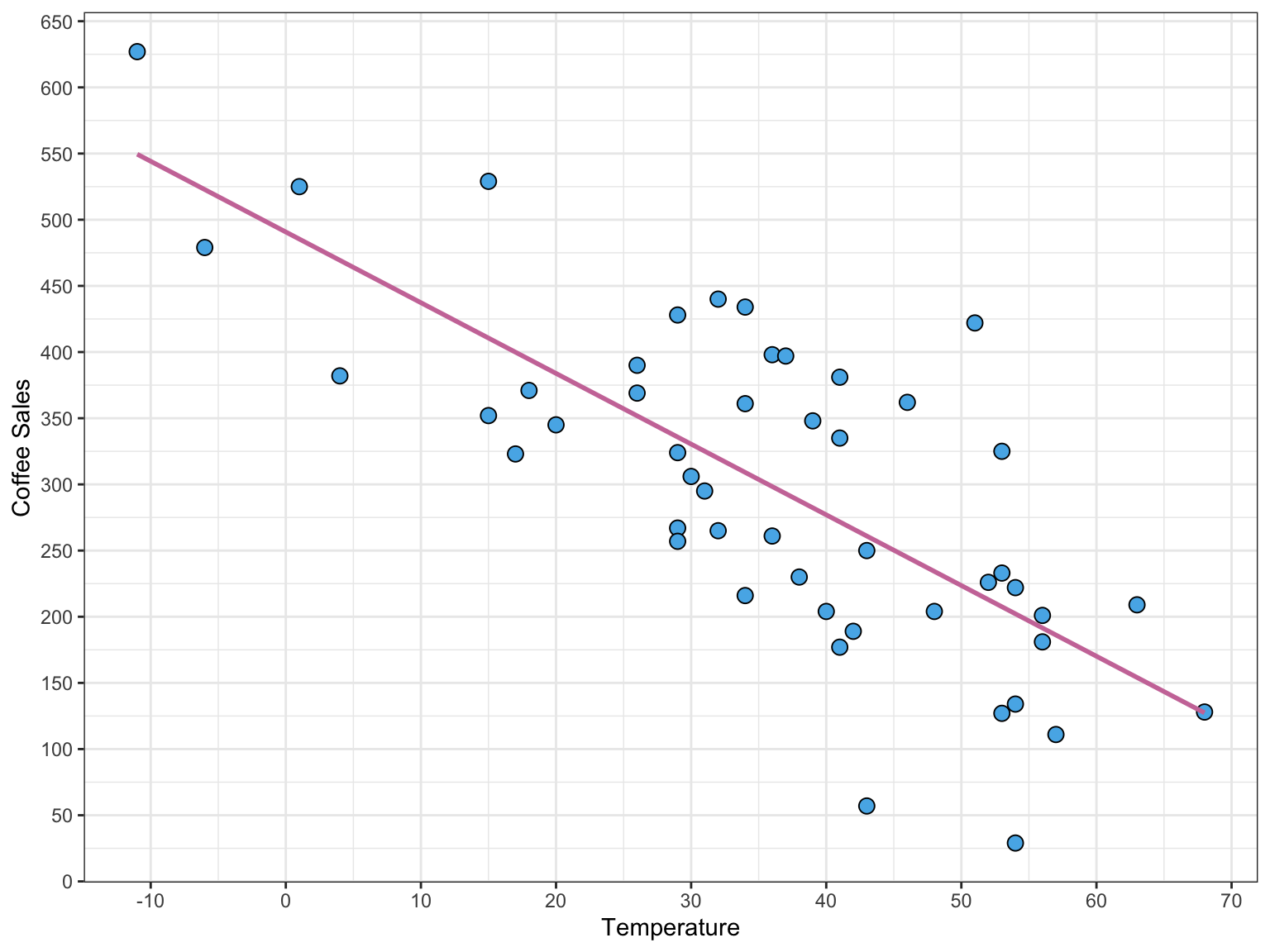
lm.a = lm(coffee_sales ~ 1 + temperature, data = coffee)
# Print regression results
lm.a

Call:
lm(formula = coffee_sales ~ 1 + temperature, data = coffee)

Coefficients:
(Intercept)  temperature  
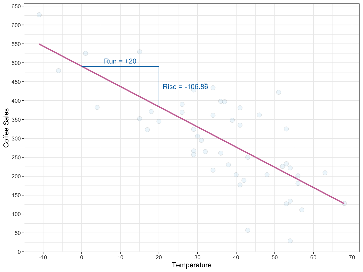
    490.729       -5.343  

Interpreting the Intercept

  • Intercept = 491
  • Where the regression line crosses y-axis at (\(X=0\))
  • Interpretation: For a 0°F day, we predict an average of 491 coffees to be sold.

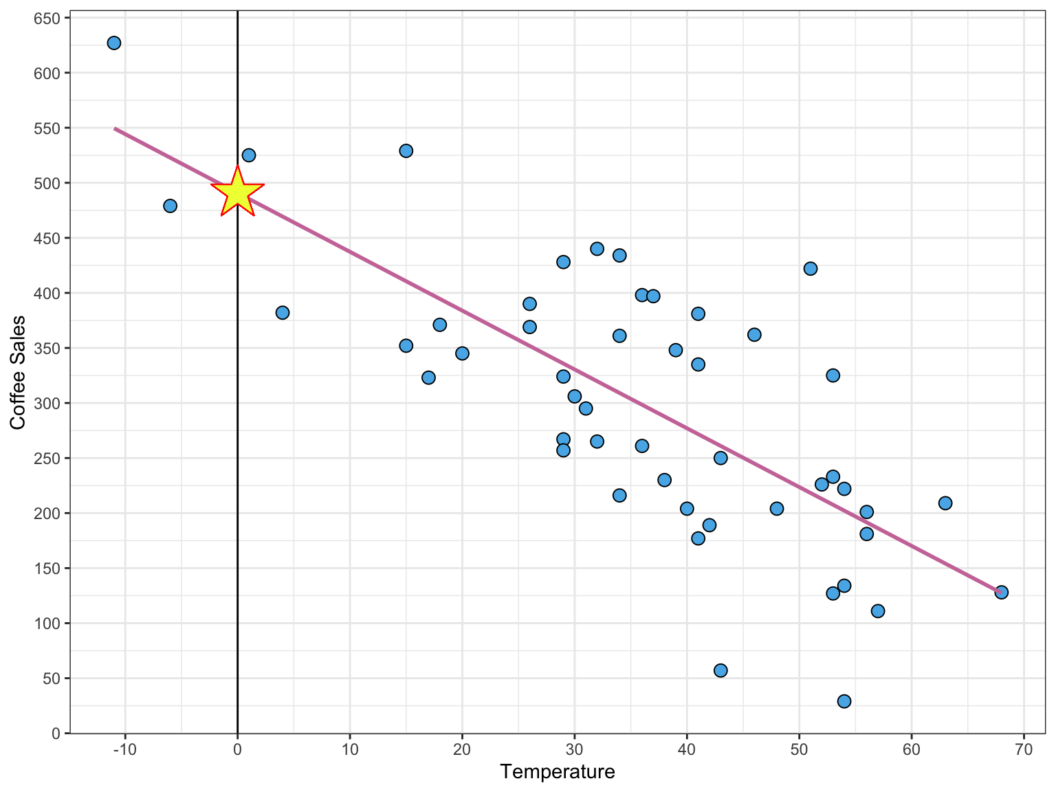
Caution: We shouldn’t interpret an intercept if 0 is not within range of data (extrapolation).

Interpreting the Slope

  • \(\text{Slope} = \frac{\text{Rise}}{\text{Run}} = \frac{\Delta Y}{\Delta X}\)
  • Predicted change in Y as X increases by 1 unit.
  • Interpretation: For each additional degree of temperature, we expect about 5.3 fewer coffees to be sold, on average.

Making Predictions Using Our Line

  • First: Beware of extrapolation!
  • Extrapolation is predicting Y values using X values that are outside the range of the data used to fit the regression. (NOT OK)
  • Can we predict coffee sales for:
    • 40 degree days?
    • 80 degree days?
    • 0 degree days?

Making Predictions Using Our Line (cntd.)

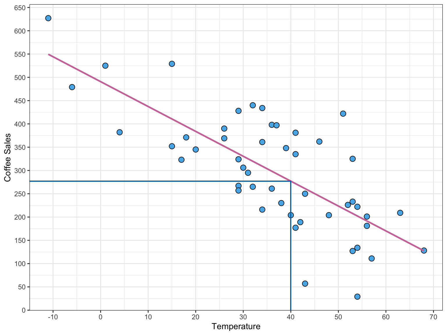
Predict about how many coffee sales to expect on a 40 degree day:

\[ \begin{split} \hat{y} &= 491 - 5.3*(40)\\ &= 279 \end{split} \]

We predict 279 coffees will be sold on a 40°day, on average.

Model Fit

Residuals

  • Residual (a.k.a. error, e) Difference between the observed and predicted values

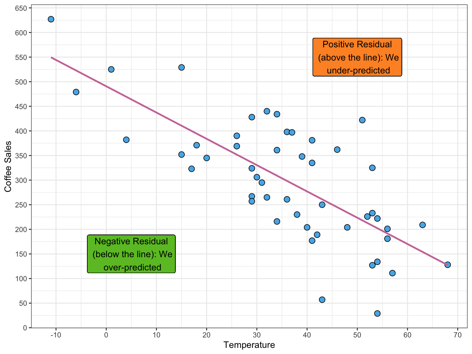
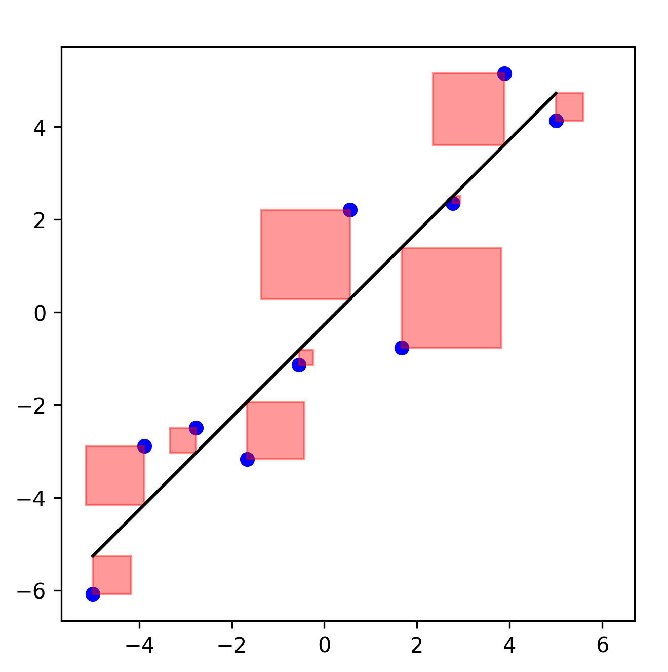
\[ \begin{split} &e = y - \hat{y}\\ &{\text{(in that order!)}} \end{split} \]

Residuals (Example)

  • On a 40 degree day we predicted to sell 27,296 coffees on a 40°day. This is our \(\hat{y}\) value.
  • Suppose we actually observed 27,100 (y) coffees were sold.
  • What is the residual?
    • Residual = \(27,100 - 27,296 = -196\)
    • The linear model over-predicted the number of coffees sold by 196.

Coefficient of Determination (\(R^2\))

  • \(R^2\) = correlation squared
  • \(R^2 = 0.741^2 = 0.549\) for coffee data
  • Idea of \(R^2\): Coffee sales vary…how much of this variation can be explained by the linear relationship with temperature?
    • 54.9% of the variation in coffee sales is explained by the linear relationship with temperature
  • \(R^2\) quantifies how much of the total variability in our response variable (Y) can be explained by this linear regression on X.

Introduction to Linear Regression Activity

Summary

  • We can create a least squares regression line to summarize the relationship between two quantitative variables.
  • We can interpret the slope and intercept of that line to describe that relationship.
  • We can use the regression line to make predictions.
  • We can use the \(R^2\) value to tell us how much variability we are explaining in the Y variable be creating a linear regression with X.