A Regression Example
In this document we will use the data in contraception.csv to examine whether female education level explains variation in contraceptive useage after controlling for GNI.
# Load libraries
library(tidyverse)
library(ggExtra)
library(broom)

# Import data
contraception = read_csv("https://github.com/zief0002/epsy-8264/raw/master/data/contraception.csv")

# View data
contraception
# IF you want to see all the variables
#print(contraception, width = Inf)Examine the Data
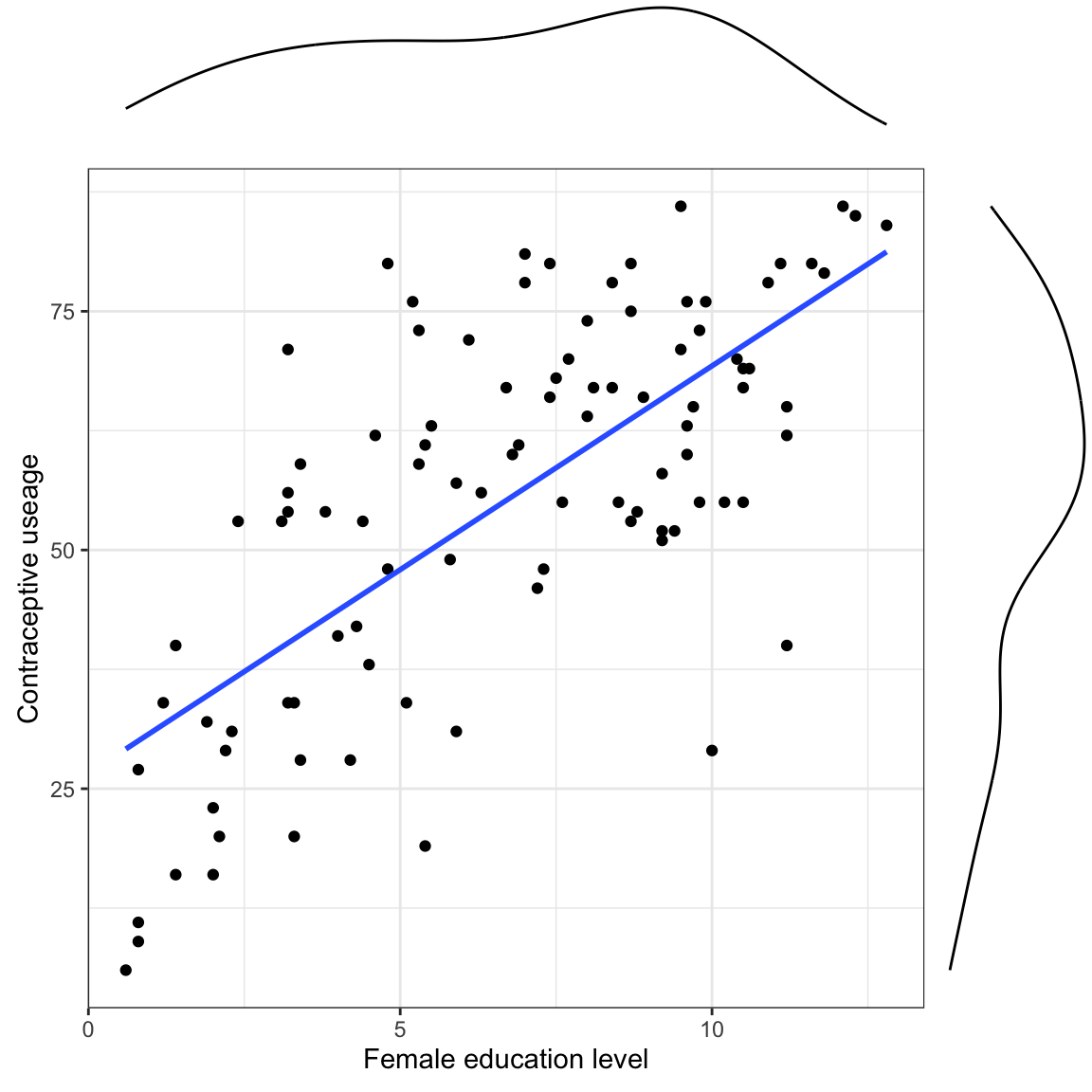
We need to correctly specify the model. Since we have no theory to guide us, this is done empirically by looking at the data.
# Create scatterplot
p = ggplot(data = contraception, aes(x = educ_female, y = contraceptive)) +
   geom_point() +
   geom_smooth(method = "lm", se = FALSE) +
   theme_bw() +
   labs(
      x = "Female education level",
      y = "Contraceptive useage"
   )

# Add marginal density plots
ggMarginal(p, type = "density")

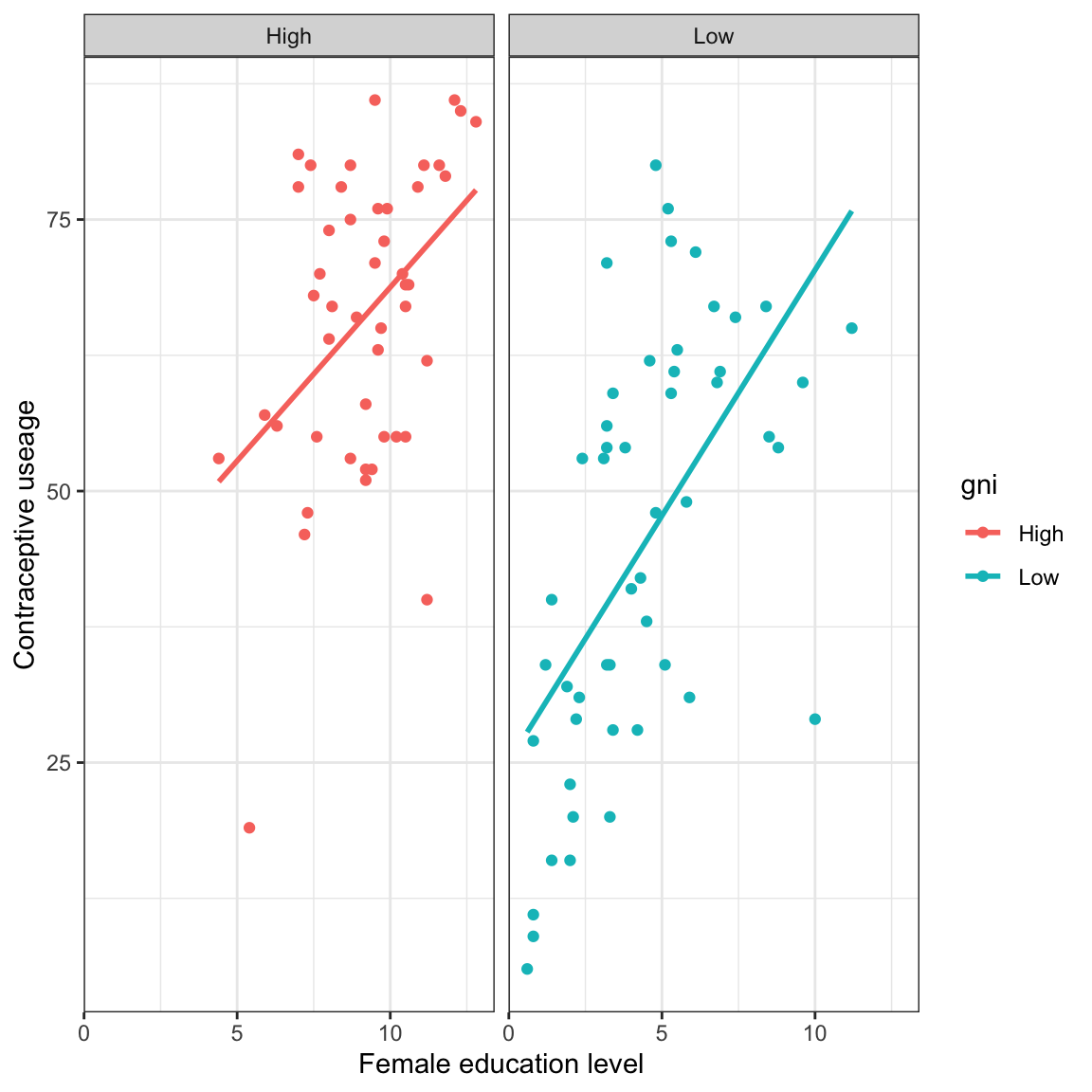
# Condition the relationship on GNI
ggplot(data = contraception, aes(x = educ_female, y = contraceptive, color = gni)) +
   geom_point() +
   geom_smooth(method = "lm", se = FALSE) +
   theme_bw() +
   labs(
      x = "Female education level",
      y = "Contraceptive useage"
   ) +
   facet_wrap(~gni)

- Should we include main-effects only? Or an interaction?
- Is there non-linearity to account for (e.g., transformations)? Or does it look linear?
Use Matrix Algebra to Compute Coefficient Estimates
\[ \mathbf{b} = (\mathbf{X}^\intercal\mathbf{X})^{-1} \mathbf{X}^\intercal\mathbf{y} \]
# Store values
n = nrow(contraception) #Sample size
k = 2 #Number of predictors


# Create outcome vector
y = contraception$contraceptive

# Create dummy variable for GNI
contraception = contraception %>%
   mutate(
      high_gni = if_else(gni == "High", 1, 0)
      )

# Create design matrix
X = matrix(
   data = c(rep(1, n), contraception$educ_female, contraception$high_gni),
   ncol = 3
)

# Compute b vector
b = solve(t(X) %*% X) %*% t(X) %*% y
b
[,1]
[1,] 27.021387
[2,] 4.088735
[3,] 1.608766Thus the fitted regression equation is:
\[ \widehat{\mathrm{Contraceptive~Use}}_i = 27.02 + 4.09(\mathrm{Female~Education~Level}_i) + 1.60(\mathrm{High~GNI}_i) \]
Compute Residual Standard Error
# Compute e vector
e = y - X %*% b

# Compute s_e
s_e = sqrt((t(e) %*% e) / (n - k - 1))
s_e
[,1]
[1,] 14.39792Thus the residual standard error (a.k.a., the root mean square error; RMSE) is:
\[ s_e = 14.40 \]
Compute Variance–Covariance Matrix for the Coefficients
\[ \mathrm{Var}(\mathbf{b}) = s^2_e(\mathbf{X}^\intercal\mathbf{X})^{-1} \]
where \(s^2_e = \frac{\mathbf{e}^\intercal\mathbf{e}}{n-k-1}\)
# Compute varaince-covariance matrix of b
V = as.numeric(s_e^2) * solve(t(X) %*% X)
V
[,1] [,2] [,3]
[1,] 12.414688 -1.8783934 4.782603
[2,] -1.878393 0.4267136 -2.028306
[3,] 4.782603 -2.0283060 18.197825# Compute SEs for b
sqrt(diag(V))[1] 3.5234483 0.6532332 4.2658909Thus
\[ \mathrm{SE}(b_0) = 3.52 \qquad \mathrm{SE}(b_1) = 0.65 \qquad \mathrm{SE}(b_2) = 4.27 \]
Coefficient-Level Inference
Here we will focus on the effects of female education level since it is our focal predictor. (GNI is a control.) Note this is the second effect in the b vector and in the V matrix. We will test the hypothesis:
\[ H_0: \beta_{\mathrm{Education}} = 0 \]
# Compute t-value
t_0 = (b[2] - 0) / sqrt(V[2, 2])
t_0
[1] 6.259228# Evaluate t-value
df = n - k - 1
p = 2* (1 - pt(abs(t_0), df = df))
p[1] 0.00000001143799Here,
\[ t(94) = 6.26,~p=0.0000000114 \]
The evidence suggests that the data are not very compatible with the hypothesis that there is no effect of female education level on contraceptive useage, after controlling for differences in GNI.
Statistical Inference: Confidence Intervals for the Coefficients
From the hypothesis test, we believe there is an effect of female education level on contraceptive useage, after controlling for differences in GNI. What is that effect? To answer this we will compute a 95% CI for the effect of female education.
# Compute critical value
t_star = qt(.025, df = df)

# Compute CI
b[2] - abs(t_star) * sqrt(V[2, 2])
[1] 2.791725b[2] + abs(t_star) * sqrt(V[2, 2])[1] 5.385745The 95% CI indicates that the population effect of female education level on contraceptive useage, after controlling for differences in GNI is between 2.79 and 5.39.
ANOVA Decompostion
Here we want to partition the sums of squares:
\[ \mathrm{SS}_{\mathrm{Total}} = \mathrm{SS}_{\mathrm{Model}} + \mathrm{SS}_{\mathrm{Residual}} \]
# Compute needed values
mean_y = mean(y)
hat_y = X %*% b


# Compute SS_Total
ss_total = t(y - mean_y) %*% (y - mean_y)
ss_total
[,1]
[1,] 38336.45# Compute SS_model
ss_model = t(hat_y - mean_y) %*% (hat_y - mean_y)
ss_model [,1]
[1,] 18850.25# Compute SS_residual
ss_residual = t(y - hat_y) %*% (y - hat_y)
ss_residual [,1]
[1,] 19486.2Here:
- \(\mathrm{SS}_{\mathrm{Total}}=38,336.45\)
- \(\mathrm{SS}_{\mathrm{Model}}=18,850.25\)
- \(\mathrm{SS}_{\mathrm{Residual}}=19,486.2\)
We can verify that:
\[ 38,336.45 = 18,850.25 + 19,486.2 \]
This can be used to compute the model-level \(R^2\) value.
\[ R^2 = \frac{\mathrm{SS}_{\mathrm{Model}}}{\mathrm{SS}_{\mathrm{Total}}} \]
# Compute R^2
r2 = ss_model / ss_total
r2
[,1]
[1,] 0.4917057The model explains 49.1% of the variation in contraception usage.
Model-Level Inference
Here we want to test whether the model explained variation is more than we would expect because of sampling variation, namely
\[ H_0: \rho^2=0 \]
This is equivalent to testing:
\[ H_0: \beta_{\mathrm{Female~Education}} = \beta_{\mathrm{GNI}} = 0 \]
We compute an observed F-value as:
\[ F_0 = \frac{(\mathbf{Lb}-\mathbf{c})^\intercal\big[\mathbf{L}(\mathbf{X}^\intercal\mathbf{X})^{-1}\mathbf{L}^\intercal\big]^{-1}(\mathbf{Lb}-\mathbf{c})}{q(s^2_e)} \]
# Create L (hypothesis matrix)
L = matrix(
   data = c(0, 1, 0, 0, 0, 1),
   byrow = TRUE,
   ncol = 3
)

# Create vector of hypothesized values
C = matrix(
   data = c(0, 0),
   ncol = 1
)

q = 2

F_num = t(L %*% b - C) %*% solve(L %*% solve(t(X) %*% X) %*% t(L)) %*% (L %*% b - C)
F_denom = q * s_e^2

F_0 = F_num / F_denom
F_0
[,1]
[1,] 45.46611# Evaluate F_0
1 - pf(F_0, df1 = q, df2 = (n - k - 1)) [,1]
[1,] 1.532108e-14Here,
\[ F(2, 94) = 45.47,~p=0.0000000000000153 \]
The data are not very compatible with the hypothesis that the model explains no variation in the outcome. It is likely there is a controlled effect of female education level, or GNI (or both) on contraceptive usage. That is, the explained variation of 49.1% is more than we would expect because of chance.
In Practice
In practice, you would simply use built-in R functions to do all of this. Note that you can use a categorical variable in the lm() function directly (without dummy coding it beforehand), but it will pick the reference category for you (alphabetically). For example:
# Fit model
lm.1 = lm(contraceptive ~ 1 + educ_female + gni, data = contraception)

# Coefficient-level output
tidy(lm.1)
# Coempute confidence intervals for coefficients
confint(lm.1) 2.5 % 97.5 %
(Intercept) 16.044734 41.215571
educ_female 2.791725 5.385745
gniLow -10.078792 6.861261# Model-level output
glance(lm.1)# ANOVA decomposition
anova(lm.1)Accessing Regression Matrices from lm()
There are several built-in R functions that allow you to access different regression matrices once you have fitted a model with lm().
# Access design matrix
model.matrix(lm.1)
(Intercept) educ_female gniLow
1 1 5.9 0
2 1 8.9 0
3 1 10.5 0
4 1 4.6 1
: : : :
97 1 6.7 1
attr(,"assign")
[1] 0 1 2
attr(,"contrasts")
attr(,"contrasts")$gni
[1] "contr.treatment"The design matrix is given and information about this design matrix is also encoded. There is an attribute “assign”, an integer vector with an entry for each column in the matrix giving the term in the formula which gave rise to the column. Value 0 corresponds to the intercept (if any), and positive values to terms in the order given by the term.labels attribute of the terms structure corresponding to object. There is also an attribute called “contrasts” that identifies any factors (categorical variables) in the model and indicates how the contrast testing (comparison of the factor levels) will be carried out. Here “contr.treatment” is used. This compares each level of the factor to the baseline (which is how dummy coding works).
# Access coefficient estimates
coef(lm.1)
(Intercept) educ_female gniLow
28.630153 4.088735 -1.608766 # Access variance-covariance matrix for b
vcov(lm.1) (Intercept) educ_female gniLow
(Intercept) 40.177719 -3.9066994 -22.980428
educ_female -3.906699 0.4267136 2.028306
gniLow -22.980428 2.0283060 18.197825# Access fitted values
fitted(lm.1) 1 2 3 4 5 6 7 8
52.75369 65.01990 71.56187 45.82957 71.56187 66.24652 35.19886 61.36676
9 10 11 12 13 14 15 16
58.06905 64.20215 71.97075 34.78998 36.01660 40.10534 47.87394 78.92160
17 18 19 20 21 22 23 24
29.47463 67.88201 57.25130 35.60773 62.97553 71.56187 78.10385 60.11341
25 26 27 28 29 30 31 32
58.88679 48.69168 51.96267 32.74562 73.19737 51.14493 69.10863 30.29238
33 34 35 36 37 38 39 40
40.10534 48.69168 74.42399 40.10534 55.23366 46.62059 68.29089 68.69976
41 42 43 44 45 46 47 48
74.42399 67.06427 70.33525 49.10056 74.01512 42.55858 59.70454 54.82479
49 50 51 52 53 54 55 56
36.42548 46.64732 40.92309 66.24652 50.70932 32.74562 67.47314 61.34004
57 58 59 60 61 62 63 64
61.74891 66.27325 61.77564 40.10534 30.29238 54.38919 36.83435 46.64732
65 66 67 68 69 70 71 72
30.29238 44.19408 40.51421 67.88201 59.29567 63.00226 61.34004 71.15300
73 74 75 76 77 78 79 80
39.69647 43.37633 40.92309 66.24652 35.19886 76.05948 76.87723 68.69976
81 82 83 84 85 86 87 88
67.47314 58.47792 57.27803 67.90874 45.42070 57.25130 40.51421 49.50943
89 90 91 92 93 94 95 96
44.60295 72.81522 80.96597 64.20215 64.20215 48.28281 31.92787 50.73605
97
54.41591 # Access raw residuals
resid(lm.1) 1 2 3 4 5 6
4.2463087 0.9801026 -16.5618739 16.1704304 -4.5618739 -15.2465180
7 8 9 10 11 12
-19.1988577 5.6332361 -12.0690473 -11.2021503 -2.9707474 -2.7899842
13 14 15 16 17 18
-7.0166048 15.8946599 -13.8739373 6.0784025 -23.4746282 8.1179879
19 20 21 22 23 24
23.7486998 -15.6077312 15.0244703 -2.5618739 7.8961495 9.8865851
25 26 27 28 29 30
21.1132057 10.3083157 20.0373274 7.2543835 4.8026319 -20.1449256
31 32 33 34 35 36
6.8913673 -21.2923753 -6.1053401 24.3083157 -12.4239887 13.8946599
37 38 39 40 41 42
5.7663391 6.3794117 -3.2908856 4.3002408 -34.4239887 -15.0642650
43 44 45 46 47 48
-15.3352533 11.8994421 5.9848849 11.4414187 -4.7045414 5.1752126
49 50 51 52 53 54
-5.4254783 1.3526833 18.0769128 -14.2465180 -31.7093236 -16.7456165
55 56 57 58 59 60
18.5268614 2.6599645 5.2510909 -6.2732463 -6.7756375 30.8946599
61 62 63 64 65 66
-3.2923753 1.6108145 16.1656482 33.3526833 -19.2923753 -16.1940755
67 68 69 70 71 72
-6.5142136 -4.8820121 8.7043321 -9.0022581 12.6599645 -1.1530004
73 74 75 76 77 78
13.3035334 -2.3763284 -12.9230872 -8.2465180 -12.1988577 3.9405172
79 80 81 82 83 84
2.1227701 -13.6997592 3.5268614 -10.4779208 8.7219714 -38.9087405
85 86 87 88 89 90
-7.4206961 20.7486998 -20.5142136 13.4905686 -2.6029490 -7.8152229
91 92 93 94 95 96
3.0340348 15.7978497 10.7978497 27.7171892 2.0721306 -1.7360520
97
12.5840862