fertility = read_csv("data/fertility.csv")📖 Introduction to Quarto
In this set of notes, you will continue your Quarto journey. One important note before we begin:
In EPsy 8251, when we create objects, they are stored in the R environment and we can operate on those objects. For example, in this document we will read in the fertility.csv data and assign it to the object fertility. We can then use functions to compute values and operate on the data.
Trying to operate on an object that we created in the R environment, but do not create in our Quarto document will lead to an error. This is because the R environment and your Quarto document are completely independent from one another.
If you want to operate on an object you have to create the object in the Quarto document.
Your First Task
To begin:
- Open the Assignment 1 R project (
assignment-01.Rproj) you created. - Create a new Quarto document called
assignment-01.qmdand save this in your root directory. The tree for your project should now look like this:
assignment-01
    ├── README
    ├── assets
    ├── assignment-01.qmd
    ├── assignment-01.Rproj
    ├── data
    │   └── fertility.csv
    ├── figs
    └── scripts
Before we start updating the document, here is a useful resource.
- If you are using the
Sourceeditor, there is a Markdown Reference Guide available in RStudio viaHelp > Markdown Quick Reference. This will include the Markdown syntax for basic things like changing the font style, creating lists, adding links, etc.
Update the YAML
In the assignment-01.qmd file, update the YAML to the following:
---
title: "Assignment 1"
subtitle: "Introduction to Quarto"
author: "Your Group's Names"
date: "January XX, 2023"
format: html
editor: visual
---
Change the date: key to today’s date. For the editor: key you can choose visual or source depending on whether you want the document to open with the visual editor or the source editor.
Adding Text
Start by clearing all the text in the document below the YAML (underneath the three hyphens). Then add some text into your document. Within this text, make some words italics and some words bold. Also add a bulletted list. (Maybe the names of the pets/plants/kids for everyone in your group.)
Adding Headings
Add a Level-1 and a Level-2 heading into your document. Separate each of these by adding some text after each of them. If you need a refresher, see the “Headings” section in the Markdown Basics Tutorial.
Code Chunks
Recall from the Computations Tutorial, we can add R syntax to our document using a code chunk.
Add a Code Chunk to Load Libraries and Import Data
The first question on Assignment 1 is:
Import the data and display the first several rows of data (not all of it). Use one of the paged table options in your YAML to ensure that this is printed nicely. All syntax for these commands should be hidden.
- Create a Level-2 Heading in your QMD document that is called “Question 1”.
- Then create a new R chunk. In that chunk load the
{tidyverse}library. Don’t forget to add a comment. - In the same R chunk, import the
fertility.csvdata into an object calledfertility.
To import the data (which you put in the data directory of your project last class) use the following syntax:
The path inside the quotation marks gives the location (relative to the QMD file) of the fertility.csv data. Here, the data are in the directory called data. Thus the path data/fertility.csv indicates go to the data folder and inside of that locate fertility.csv.
What would the path be inside the quotation marks if our project had the following tree?
assignment-01
    ├── README
    ├── assets
    ├── assignment-01.qmd
    ├── assignment-01.Rproj
    ├── data
       ├── assignment-data
          └── fertility.csv
       └── notes-data
    ├── figs
    └── scripts
Use the first code chunk in your Quarto document to load all the packages and datasets used in the document. Label this chunk setup. This has the added advantage that others can immediately see what packages and datasets are needed to run the document. Labelling it setup also runs that chunk when you try to run other chunks, so your code works!
Displaying Data
In the same R chunk display the data by typing the data object name after you import the data.
Rendering the document should display the entire data set in your outputted HTML file! In general, we do not want to take the space (especially when data sets are large) to do this. One option is to change the way that data frames/tibbles are printed in the Quarto document. To do this we need to update our YAML.
Update the YAML of your QMD to the following:
---
title: "Assignment 1"
subtitle: "Introduction to Quarto"
author: "Your Group's Names"
date: "January XX, 2023"
format:
  html:
    df-print: paged
editor: visual
---
Re-render the document.
This sets the printing option for data frames into an HTML table that has clickable paging when the data are large. The Quarto documentation Data Frames, includes other options for printing data frames.
Pay attention to the spacing in the YAML!!!!
Add a Code Chunk to Create a Plot
Create another Level-1 header in your document called “Scatterplot”. Then create a code chunk in which you create a scatterplot of infant mortality rates (y-axis) versus female education level (x-axis).
It is a good idea to include a label in the chunk options for each plot you create. A label is the name of this code chunk. (Any code chunk, even if it is not a plot, can have a label.) In the plot below, the chunk’s label is fig-scatterplot.
```{r}
#| label: fig-scatterplot
#| fig-cap: "Scatterplot showing the relationship between female education level and infant mortality."
ggplot(data = fertility, aes(x = educ_female, y = infant_mortality)) +
   geom_point()
```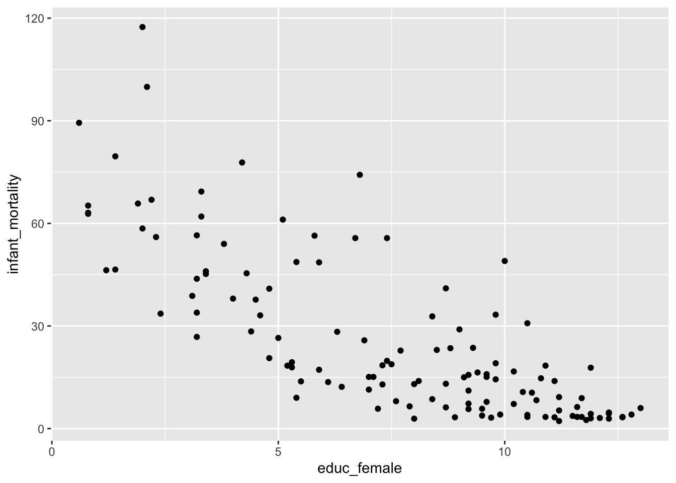
Notice that by labeling this chunk, the figure is numbered in the document. We also added a caption using the fig-cap: option.
Figure Size
There are a couple other chunk options for figures that help set the aspect ratio and size of the figure in your document. The aspect ratio is the ratio of a figure’s width to its height. We set this using the fig-width: and fig-height: chunk options. (The default value for both is 6; thus the figure appears square.) Below we change these so that the figure appears wider than it is tall.
```{r}
#| label: fig-scatterplot-2
#| fig-cap: "Scatterplot showing the relationship between female education level and infant mortality."
#| fig-width: 9
#| fig-height: 5
ggplot(data = fertility, aes(x = educ_female, y = infant_mortality)) +
   geom_point()
```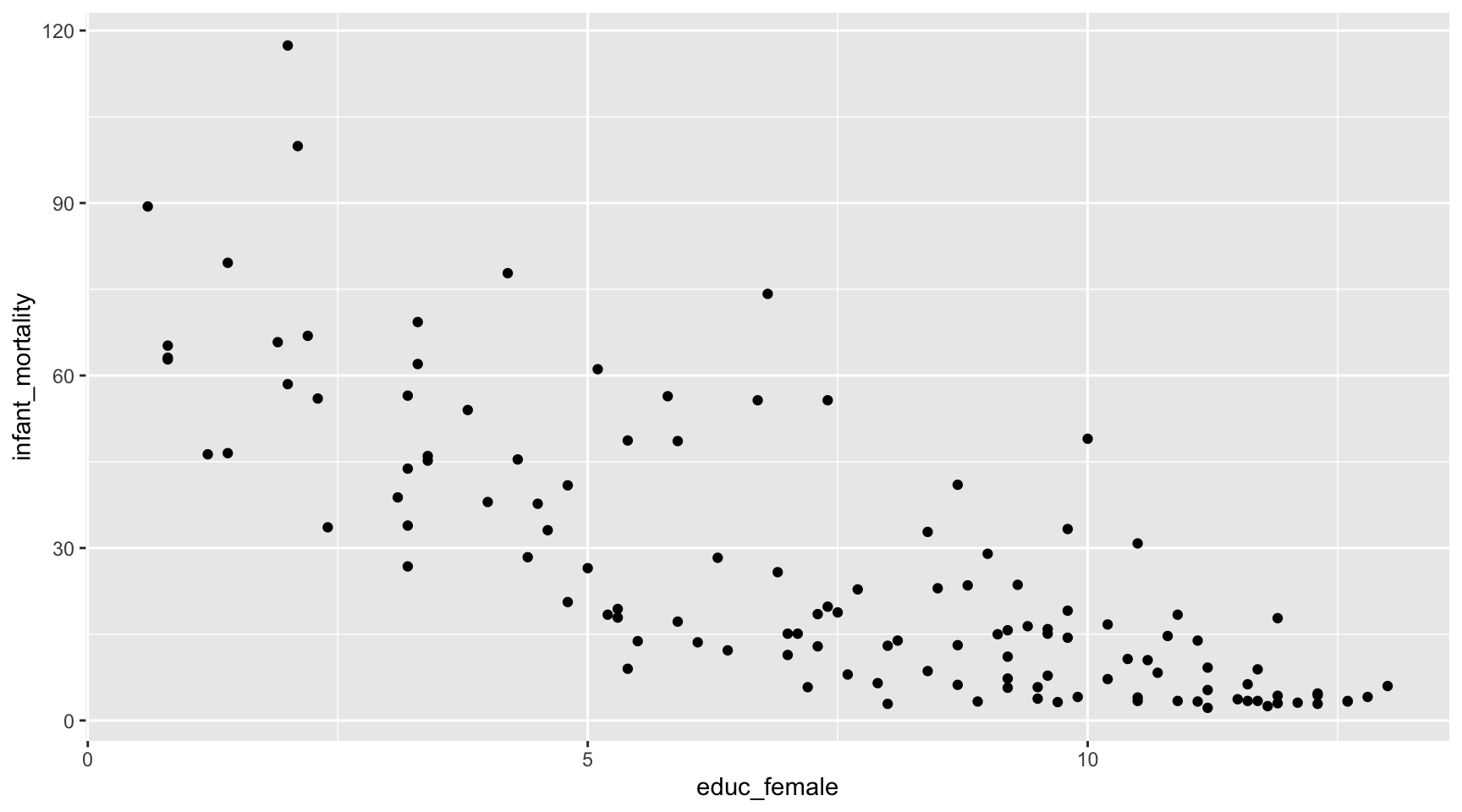
It is important to change the aspect ratio when you have legends or when you are using {patchwork} to stack or put multiple figures next to each other. Many times you need to find a good aspect ratio though trial-and-error of trying different values.
The actual size of the figure in the document is independent of the aspect ratio and can be set using the out-width: or out-height: chunk option. These options take a character string of the direct size (in HTML documents this is typically in pixels) or of the percentage of the output width/height. Here we keep the same aspect ratio, but make the figure smaller by setting the figure width to 40% of the document’s width.
```{r}
#| label: fig-scatterplot-3
#| fig-cap: "Scatterplot showing the relationship between female education level and infant mortality."
#| fig-width: 9
#| fig-height: 5
#| out-width: "40%"
ggplot(data = fertility, aes(x = educ_female, y = infant_mortality)) +
   geom_point()
```
If you set the aspect ratio of the figure, you need only set out-width: or out-height:. You don’t need to set both as the other will be determined by the aspect ratio.
Inline Code Chunks for Better Reproducibility
In writing papers where there are results from data analyses being reported in the text, inline code chunks are boss! For example, consider writing the following sentence in an analysis of the fertility.csv data.
The mean infant mortality rate is 26.05% (SD = 23.98).
Rather than computing these values and then transposing the values into the sentence, we can use inline code chunks to directly compute and write the values in the sentence. Here is some syntax we could use:
The mean infant mortality rate is `r mean(fertility$infant_mortality)` (SD = `r sd(fertility$infant_mortality)`).
This produces the following sentence in the rendered document:
The mean infant mortality rate is 26.05 (SD = 23.982719).
Rounding
There are several ways to set the rounding to two decimal places. One is to embed the computation in the round() function. For example, in the first inline chunk we could use: round(mean(fertility$infant_mortality), 2).
You can also do this in a separate code chunk and then call the values in the inline computation (as suggested in the Quarto Computations Tutorial).
Equations
There are two different manners in which equations/mathematics is included in a document.
- Display equations are typeset on a separate line from the body text and are centered on the page.
- Inline equations are typeset directly within the body text.
For example, here is a display equation:
\[ y_i = \beta_0 + \beta_1(x_i) + \epsilon_i \]
The syntax I used to create this display equation is:
$$
y_i = \beta_0 + \beta_1(x_i) + \epsilon_i
$$
Here is the same equation as an inline equation: \(y_i = \beta_0 + \beta_1(x_i) + \epsilon_i\). Notice that in an inline equation, the equation is embedded directly in the text. To create the inline equation we embed the mathematical expression in single dollar signs ($y_i = \beta_0 + \beta_1(x_i) + \epsilon_i$) rather than double dollar signs.
If you need a reminder about how to create these, check out the “Equations” section of the Markdown Basics tutorial.
The syntax we use to create the mathematical expressions is from LaTeX. Here are a couple reference you can use:
Your Turn
Part of Question #8 asks you to use a display equation to write the fitted equation based on the following output.
Try to write this fitted equation in your Quarto document using a display equation.
Better Typesetting of Equations
When we typeset equations, there are a couple things we should do:
- Use variable names that make sense to our reader, rather than their name in our dataset/R. For example “Female Education Level” is a better name than “educ_female”.
This means we will need to add spaces into our variable names in the mathematical expression. If you tried that earlier, you found out that just hitting the spacebar does not produce a space in the outputted expression. We need to include a tilde (~) every time you want a space. So to get the name “Female Education Level” we need to use the following in our equation:
$$
Female~Education~Level
$$- Variable names should also be typeset using normal text rather than italic (the default in mathematical expressions).
To achieve this, we have to embed the text we want to be normal in the syntax \mathrm{}. This typesets the text in a roman font (normal text). For example:
$$
\mathrm{Female~Education~Level}
$$
You can also use \mathit{} (italics), \mathbf{} (bold), \mathtt{} (typewriter text), and \mathcal{} (caligraphy; this is useful for the “N” we use to indicate a normal distribution).
- Hyphens need special syntax since a hyphen would be interpreted as a minus sign. In typesetting, the minus sign is longer than the hyphen symbol.
If you want to include a hyphen, we need to include it in \mbox{}. For example, to add a hyphen in our variable name to get “Female Education-Level”, we use:
$$
\mathrm{Female~Education\mbox{-}Level}
$$
Update your fitted equation from before to include spaces in variable names. Also be sure the variable names are written in normal font.
Multiline Equations
There are a couple of ways to create multiline equations in a Quarto document. I tend to use the split environment from LaTeX to do this. To use this:
- Include
\begin{split}and\end{split}in the display equation. - At the end of each line (where you want a linebreak) include a double backslash,
\\. - In each line of the multiline equation, also include the ampersand sign (
&) at the point we want the multiple lines to align vertically.
Here is an example:
$$
\begin{split}
\hat{y}_i &= 3 + 4(1) \\
&= 7
\end{split}
$$
And the resulting display equation is:
\[ \begin{split} \hat{y}_i &= 3 + 4(1) \\ &= 7 \end{split} \]
Note that the ampersand appeared immediately before the equal sign in each line of the equation, so that is where the two lines are aligned vertically (the equal signs are on top of each other). You can add as many lines to this as you want.
Multiline equations are quite useful to show your work and when you have really long single equations that need to be broken up so they fit on the page (e.g., a regression equation with many predictors).
Spacing Out the Lines
You can add space between the lines of your multiline equation by including a unit of measurement between square brackets after the double backslashes.
$$
\begin{split}
\hat{y}_i &= 3 + 4(1) \\[1em]
&= 7
\end{split}
$$
Here the resulting display equation is:
\[ \begin{split} \hat{y}_i &= 3 + 4(1) \\[1em] &= 7 \end{split} \]
Here we have added line space of 1 em. An em is a unit for measuring the width of printed work, equal to the height of the type size being used (typically the width of the letter “m”). Other common printing units include the en (the width of the letter “n”), and the ex (the width of the letter “x”).
Question #8 actually asks:
Use a display equation to write the equation for the underlying regression model (including error and assumptions) using Greek letters, subscripts, and variable names. Also write the equation for the fitted least squares regression equation based on the output from
lm(). Type these two equations in the same display equation, each on a separate line of text in your document, and align the equals signs.
Try writing this multiline equation.
Hyphens, Minus Signs, and Dashes
In printed work the width of a hyphen, a minus sign, and dashes are all different. Quarto will correctly typeset these, but you have to indicate what you want. Below are how we indicate these in Quarto.
- Hyphen: A hyphen is used to join two or more words together. To typeset a hyphen in Quarto, use a single hyphen;
-. - En Dash: An en dash is used to mark ranges and to indicate the meaning “to” in phrases like “Minneapolis–St. Paul”. An en dash is slightly longer than a hyphen and is typeset in Quarto using two hyphens;
--. - Em Dash: An em dash is used to separate extra information or mark a break in a sentence. An em dash is slightly longer than an en dash and is typeset in Quarto using three hyphens;
---. - Minus Sign: A minus sign is used in mathematical expressions (e.g., in subtraction or to indicate a negative number). To typeset a minus sign, use the inline equation with a single hyphen;
$-$. When a minus sign is typeset, not only is the length of it different than a hyphen, but it also includes the correct spacing around it for mathematical typesetting.
Here is a sentence incorporating each of these so you can see the differences:
During the time from January–February, my three dogs enjoy playing in the snow—apparently snow is fun for canines—with their sweaters on since it is \(-30\)-degrees Fahrenheit outside.
The input for this sentence was:
During the time from January--February, my three dogs enjoy playing in the snow---apparently snow is fun for canines---with their sweaters on since it is $-30$-degrees Fahrenheit outside.
Note that you can also typeset these in Word:
- Hyphen: On both a Mac and PC, press “hyphen”.
- En Dash: On a Mac, press “option+hyphen key”. On a PC, press “ctrl+hyphen”.
- Em Dash: On a Mac, press “option+shift+hyphen key”. On a PC, press “alt+ctrl+hyphen”.
- Minus Sign: For a minus sign, you should use Equation Editor.