More Logistic Regression
Preparation
In this set of notes, you will expand your knowledge of the logistic regression model to include non-linear predictor effects, covariates, and interaction terms. We will again use data from the file graduation.csv to explore predictors of college graduation.
Within the analysis, we will focus on the research question of whether the probability of obtaining a degree differs for first and non-first generation students. We will use information criteria as the framework of evidence to adopt different models, along with an evaluation of the models’ residuals.
# Load libraries
library(AICcmodavg)
library(broom)
library(corrr)
library(patchwork)
library(performance)
library(texreg)
library(tidyverse)

# Read in data and create dummy variable for categorical variables
grad = read_csv(file = "https://raw.githubusercontent.com/zief0002/bespectacled-antelope/main/data/graduation.csv") |>
  mutate(
    got_degree = if_else(degree == "Yes", 1, 0),
    is_firstgen = if_else(first_gen == "Yes", 1, 0),
    is_nontrad = if_else(non_traditional == "Yes", 1, 0),
  )

# View data
grad
# Fit models from previous notes
glm.0 = glm(got_degree ~ 1, data = grad, family = binomial(link = "logit"))
glm.1 = glm(got_degree ~ 1 + act, data = grad, family = binomial(link = "logit"))
glm.2 = glm(got_degree ~ 1 + is_firstgen, data = grad, family = binomial(link = "logit"))The results from glm.2 indicated that there were differences between first and non-first generation students in the probability of obtaining a degree. Based on this model’s result, we found that the predicted probability of obtaining a degre for first generation students was 0.780 while that for non-first generation students was 0.622. Does this difference persist after controlling for other covariates?
To examine this, we want to fit a set of models that systematically include potential covariates along with first generation status. Our strategy for this is to start with the most important covariate. We can compare the model that includes first generation status and this covariate to a model that just includes first generation status. If the evidence indicates that the model with only first generation status is important we are done. If the evidence points toward the model that also includes the most important covariate, then we will continue by comparing that model to one that includes first generation status and the two most important covariates. We will continue with these comparisons until we adopt a final model or models.
To determine the order of importance, we can compute the correlations between each covariate and the dummy-coded outcome.
grad |>
  select(got_degree, act, scholarship, ap_courses,is_nontrad) |>
  correlate()
The rank ordering of covariates (based on the absolute value of the correlation coefficients) will be:
- ACT scores (\(r = 0.195\), most important)
- Number of AP courses (\(r = 0.149\))
- Scholarship amount (\(r = 0.142\))
- Non-traditional status (\(r = -0.084\))
Non-Linear Effect of ACT
To begin the analysis, we will include ACT scores as a covariate in the model. Since the act variable is continuous, we need to use the “correct” functional form when we include it in the model. In the previous set of notes, we saw some misfit when we examined the binned residual plot for the logistic regression model that included ACT as a predictor of the probability of obtaining a degree. One possibility is that this may be because the effect of ACT on these probabilities is non-linear. To examine this, we can plot the empirical log-odds of obtaining a degree versus ACT scores, and examine the functional form of the relationship.
Code
# Obtain the log-odds who obtain a degree for each ACT score
prop_grad = grad |>
  group_by(act, degree) |>
  summarize(N = n()) |>
  mutate(
    Prop = N / sum (N)
    ) |>
  ungroup() |>
  filter(degree == "Yes") |>
  mutate(
    Odds = Prop / (1 - Prop),
    Logits = log(Odds)
  )

# Scatterplot
ggplot(data = prop_grad, aes(x = act, y = Logits)) +
  geom_point(aes(size = N)) +
  geom_smooth(aes(weight = N), method = "loess", se = FALSE) +
  theme_bw() +
  xlab("ACT score") +
  ylab("Log-odds of obtaining a degree")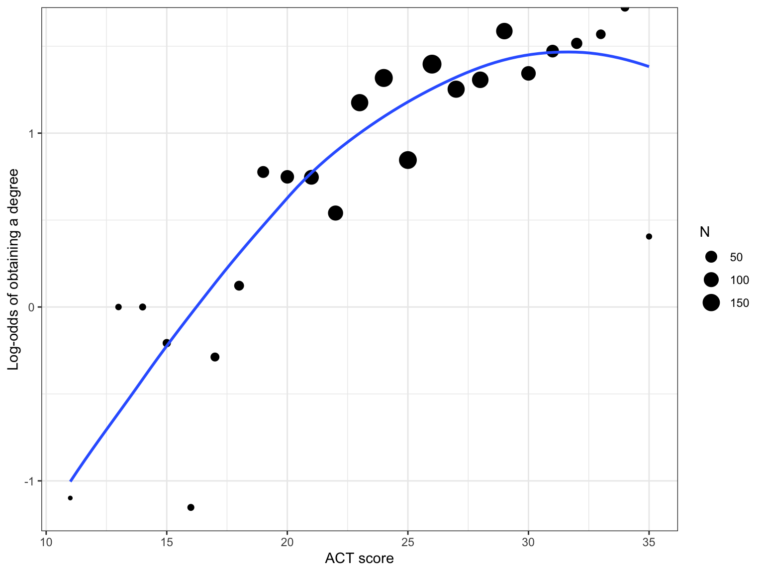
This suggests a non-linear relationship between ACT score and the log-odds of obtaining a degree. Using the Rule-of-the-Bulge, we can try to linearize this relationship by:
- Including a quadratic effect of ACT; or
- Log-transforming the ACT variable.
# Fit non-linear models
glm.1_quad = glm(got_degree ~ 1 + act + I(act^2), data = grad, family = binomial(link = "logit"))
glm.1_log = glm(got_degree ~ 1 + log(act), data = grad, family = binomial(link = "logit"))

# Obtain binned residuals
out.1_quad = binned_residuals(glm.1_quad)
out.1_log = binned_residuals(glm.1_log)

# Binned residual plots
plot(out.1_quad) | plot(out.1_log)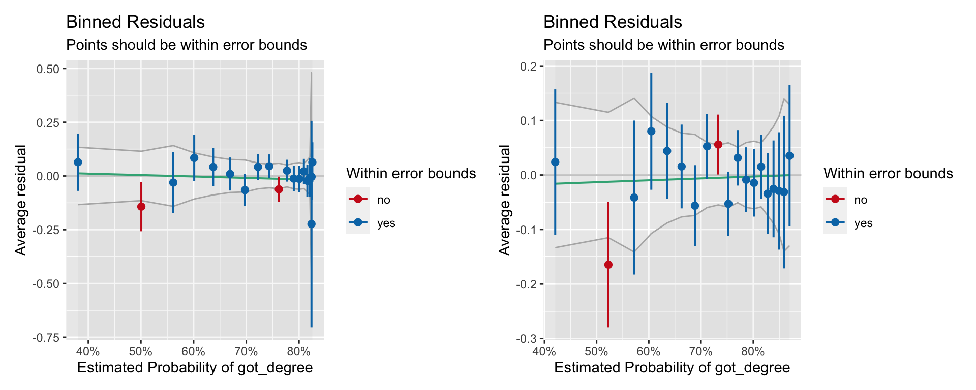
The binned residuals show slight misfit to both the log-linear model and the quadratic model. We also examine the empirical support via information criteria.
aictab(
  cand.set = list(glm.1, glm.1_quad, glm.1_log),
  modnames = c("Linear Effect", "Quadratic Effect", "Log-Linear Effect")
)
Here the most empirically supported model (given the data and the candidate models) is the quadratic model, although there is also a great deal of support for the log-linear model. I would probably adopt the log-linear model based on its simplicity and the theoretical rationale that I would not expect the probability of graduating to be smaller for high ACT values. But, for pedagogical purposes, we will look at and interpret the output for both models.
Quadratic Effect of ACT
We will start our interpretation by examining the tidy() output.
tidy(glm.1_quad)The fitted model is:
\[ \ln \bigg( \frac{\hat\pi_i}{1 - \hat\pi_i}\bigg) = -4.57 + 0.37(\mathrm{ACT}_i) - 0.005(\mathrm{ACT}_i^2) \]
Since this is an interaction model, we interpret the effect of ACT as: The effect of ACT on the log-odds of obtaining a degree depends on ACT. (We could also graph this effect if we were interested in the effect of ACT on the log-odds of obtaining a degree.)
Transforming the fitted equation to the odds metric:
\[ \frac{\hat\pi_i}{1 - \hat\pi_i} = e^{-4.57} \times e^{0.37(\mathrm{ACT}_i)} \times e^ {-0.005(\mathrm{ACT}_i^2)} \]
Because changing ACT now impacts two exponent terms, one of which includes the quadratic of ACT, it is super essential that we create a plot to interpret the effects of ACT on the odds of obtaining a degree.
# Plot the fitted equation
ggplot(data = grad, aes(x = act, y = got_degree)) +
  geom_point(alpha = 0) +
  geom_function(
    fun = function(x) {exp(-4.57 + 0.37*x - 0.005*x^2)}
    ) +
  theme_light() +
  xlab("ACT score") +
  ylab("Predicted odds of obtaining a degree")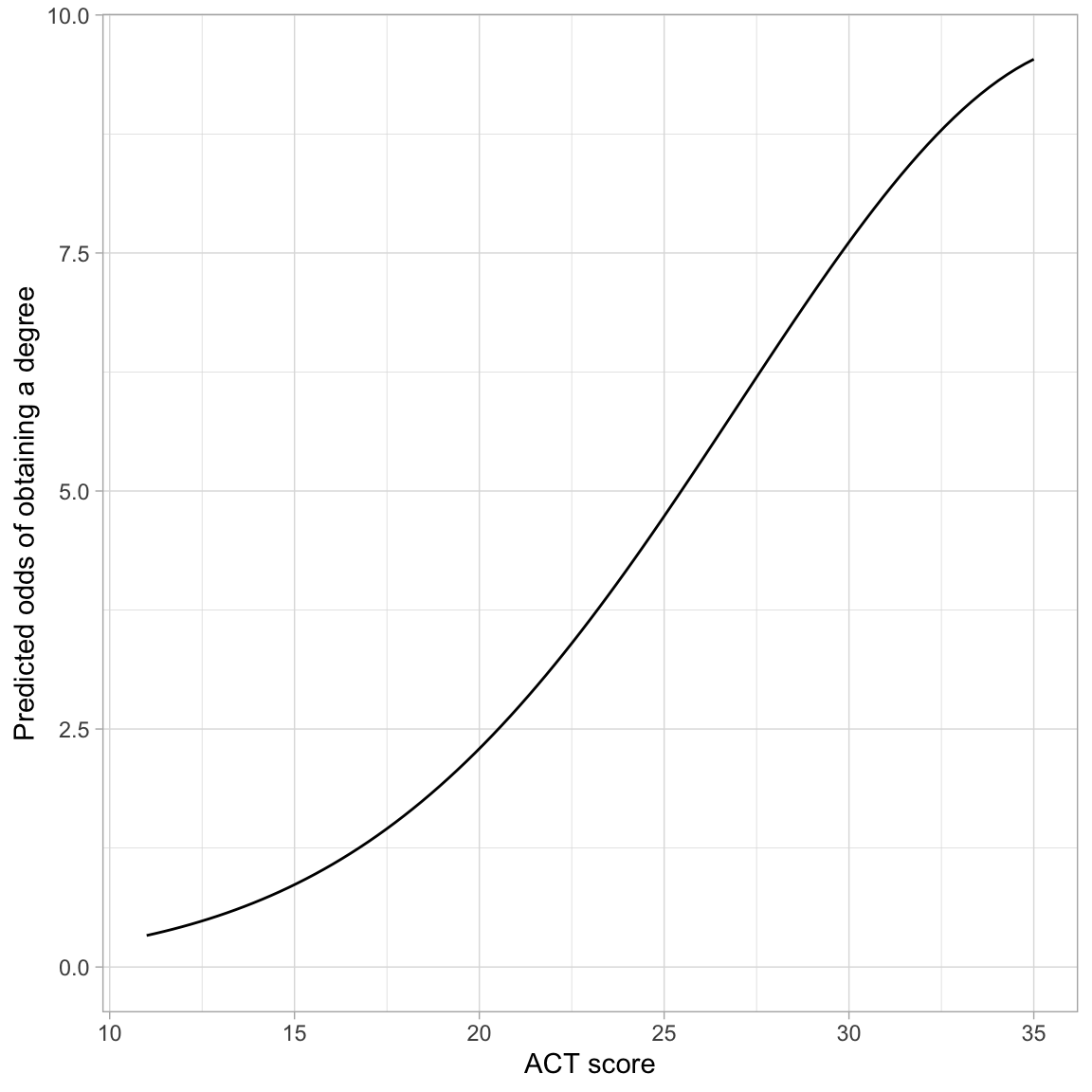
The odds curve is somewhat “S”-shaped (although it is not constrained between 0 and 1 like the probability curve). This is because of the quadratic effect of ACT. The overall trend is one of exponential growth, although the rate-of-change is not constant within this curve. The most rapid change in the odds of obtaining a degree occurs at ACT scores between 20 and 30.
Finally, we could also transform the equation into the probability metric. The fitted equation is:
\[ \hat\pi_i = \frac{e^{-4.57 + 0.37(\mathrm{ACT}_i) - 0.005(\mathrm{ACT}_i^2)}}{1 + e^{-4.57 + 0.37(\mathrm{ACT}_i) - 0.005(\mathrm{ACT}_i^2)}} \]
Again, it is worthwhile to create a plot to interpret the effects of ACT on the probability of obtaining a degree.
# Plot the fitted equation
ggplot(data = grad, aes(x = act, y = got_degree)) +
  geom_point(alpha = 0) +
  geom_function(
    fun = function(x) {exp(-4.57 + 0.37*x - 0.005*x^2) / (1 + exp(-4.57 + 0.37*x - 0.005*x^2))}
    ) +
  theme_light() +
  xlab("ACT score") +
  ylab("Predicted probability of obtaining a degree")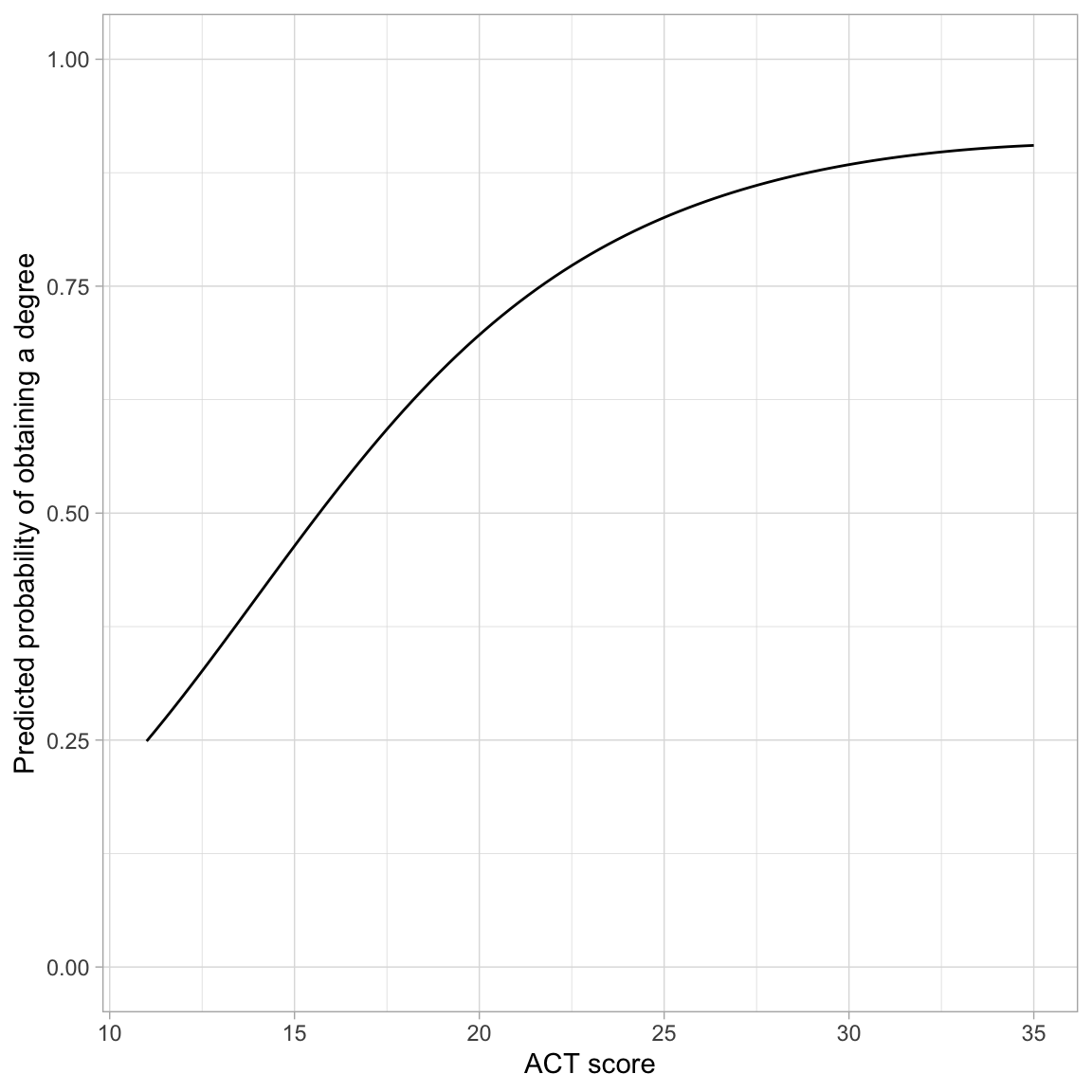
The probability curve is “S”-shaped and constrained between 0 and 1. The left-hand side of the “S” is compressed, probably due to the range of ACT scores. ACT has the largest effect on the probability of obtaining a degree for scores less than 25, and then the effect begins to plateau (although it is still growing as the logistic curve is monotonic).
Log-Linear Effect of ACT
We will again start our interpretation by examining the tidy() output.
tidy(glm.1_log)The fitted model is:
\[ \ln \bigg( \frac{\hat\pi_i}{1 - \hat\pi_i}\bigg) = -6.94 + 2.50\bigg[\ln(\mathrm{ACT}_i)\bigg] \]
We interpret the effect of ACT as: Each 1% difference in ACT score is associated with a .025-unit change in the log-odds of obtaining a degree.
Transforming the fitted equation to the odds metric:
\[ \frac{\hat\pi_i}{1 - \hat\pi_i} = e^{-6.94} \times e^{2.50\bigg[\ln(\mathrm{ACT}_i)\bigg]} \]
It is again easier to interpret the effects of ACT on the odds of obtaining a degree by creating a plot .
# Plot the fitted equation
ggplot(data = grad, aes(x = act, y = got_degree)) +
  geom_point(alpha = 0) +
  geom_function(
    fun = function(x) {exp(-6.94 + 2.50*log(x))}
    ) +
  theme_light() +
  xlab("ACT score") +
  ylab("Predicted odds of obtaining a degree")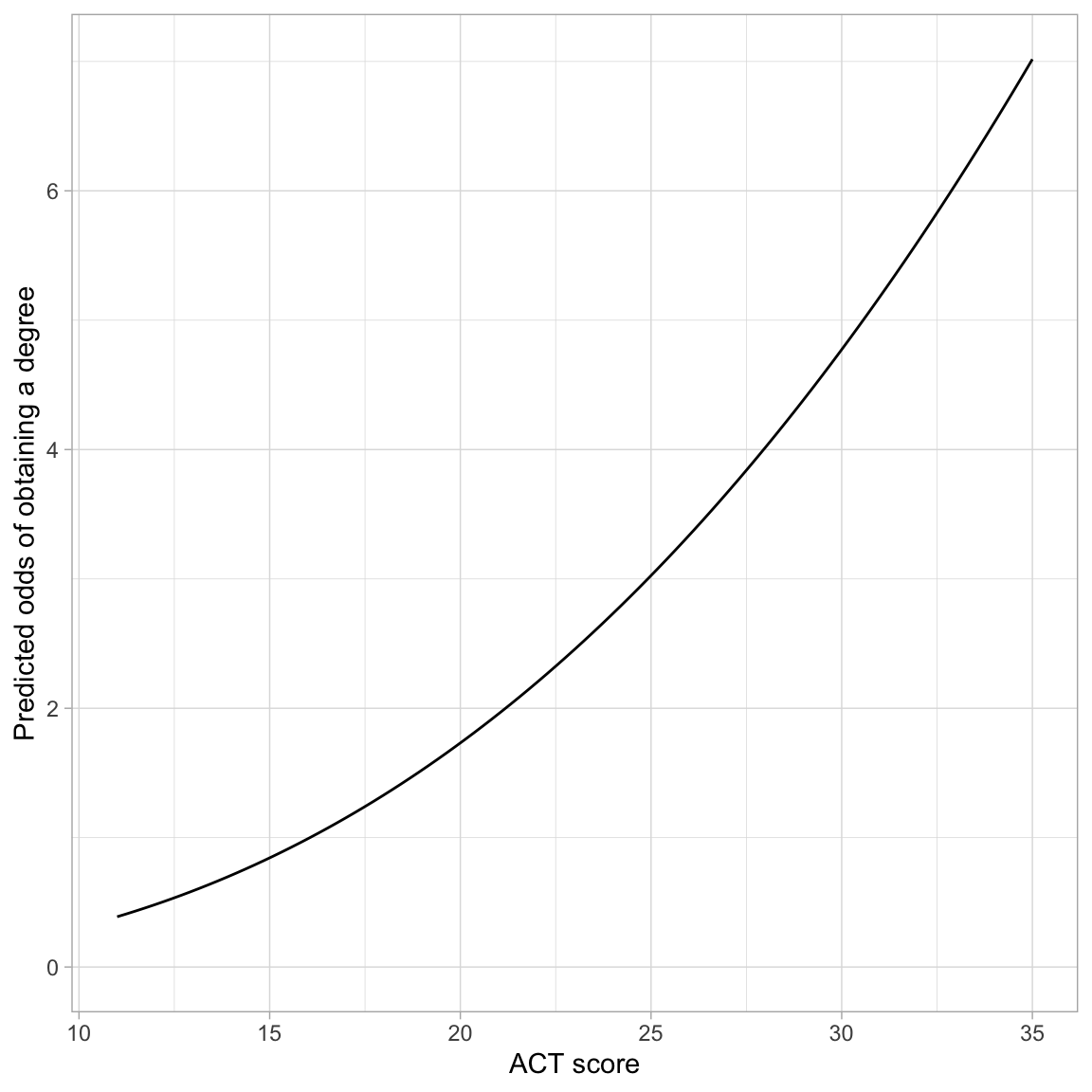
The effect of ACT on the probability of obtaining a degree is positive and non-linear (exponential growth). The predicted odds of obtaining a degree increases exponentially for higher ACT scores.
Finally, we could also transform the equation into the probability metric. The fitted equation is:
\[ \hat\pi_i = \frac{e^{-6.94 + 2.50\bigg[\ln(\mathrm{ACT}_i)\bigg]}}{1 + e^{-6.94 + 2.50\bigg[\ln(\mathrm{ACT}_i)\bigg]}} \]
Again, it is worthwhile to create a plot to interpret the effects of ACT on the probability of obtaining a degree.
# Plot the fitted equation
ggplot(data = grad, aes(x = act, y = got_degree)) +
  geom_point(alpha = 0) +
  geom_function(
    fun = function(x) {exp(-6.94 + 2.50*log(x)) / (1 + exp(-6.94 + 2.50*log(x)))}
    ) +
  theme_light() +
  xlab("ACT score") +
  ylab("Predicted probability of obtaining a degree")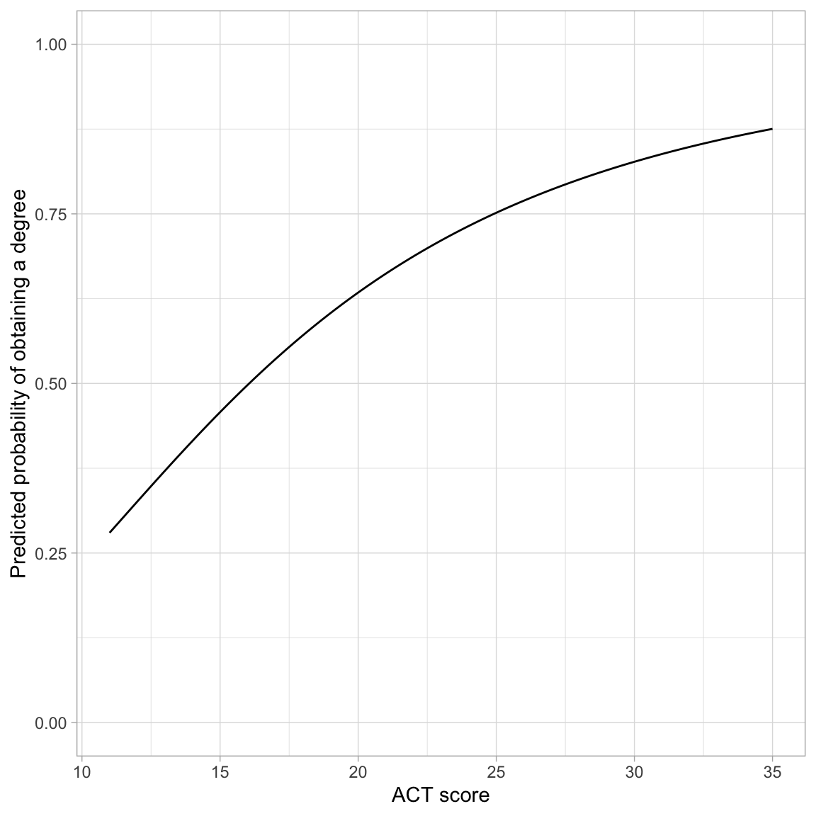
The effect of ACT on the probability of obtaining a degree is positive and non-linear. ACT has a larger effect on the probability of obtaining a degree for smaller ACT scores and this effect, while still positive, diminishes for higher ACT scores.
Once you include non-linear effects in the model, always create a plot of the fitted equation to try and interpret odds or probabilities.
Adding Covariates: Main Effects Models
Now that we have settled on a functional form for the effect of ACT, we can include it as a covariate in a model with first generation status. Including covariates in the logistic model is done the same way as for lm() models. We fit that model with the following syntax:
# Fit main effects model
glm.3 = glm(got_degree ~ 1 + is_firstgen + log(act), data = grad, family = binomial(link = "logit"))
To evaluate this model, and to begin to provide an answer for our research question, we will examine the model evidence comparing this model to both the baseline model (intercept-only) and the model that included the main-effect of first generation status.
# Model evidence
aictab(
  cand.set = list(glm.0, glm.2, glm.3),
  modnames = c("Intercept-Only", "First Gen.", "First Gen. + ACT")
)
Given the data and candidate models fitted, the empirical evidence overwhelmingly supports including both ACT scores and first generation status in the model. Adopting this model, we next look at the coefficient-level output:
# Coefficient-level output
tidy(glm.3)
The fitted equation is:
\[ \ln \bigg( \frac{\hat\pi_i}{1 - \hat\pi_i}\bigg) = -5.91 + 0.51(\mathrm{First~Generation}_i) + 2.07\bigg[\ln(\mathrm{ACT~Score}_i)\bigg] \]
Using the logit/log-odds metric, we interpret the coefficients as:
- Non-first generations students with an ACT score of 1 have a predicted log-odds of graduating of \(-5.91\).
- Each 1% difference in ACT score is associated with a difference of 0.02 in the predicted log-odds of graduating, after controlling for first generation status.
- First generation college students, have a predicted log-odds of graduating that is 0.51 higher than students who are not first generation students, after controlling for differences in ACT scores.
Back-Transforming to Odds
If we back-transform the coefficients to facilitate interpretations using the odds metric, the fitted equation is:
\[ \begin{split} \frac{\hat\pi_i}{1 - \hat\pi_i} &= e^{-5.91 + 0.51(\mathrm{First~Generation}_i) + 2.07\bigg[\ln(\mathrm{ACT~Score}_i)\bigg]} \\[1ex] &=e^{-5.91} \times e^{0.51(\mathrm{First~Generation}_i)} \times e^{2.07\bigg[\ln(\mathrm{ACT~Score}_i)\bigg]} \end{split} \]
We can interpret the intercept and the effect of first generation status directly:
- Non-first generations students with an ACT score of 1 have a predicted odds of graduating of \(e^{-5.91}=.003\).
- First generation college students, have a predicted odds of graduating that is \(e^{0.51}=1.66\) times higher than that for non-first generations students, after controlling for differences in ACT scores.
- Each one-point difference in ACT score is associated with improving the odds of graduating 1.09 times, on average, after controlling for whether or not the students are first generation college students.
While it is not pertinent to the research question, if you wanted to interpret the effect of ACT, you could plot the fitted model. As always with main effects models, we find the fitted equation for first generation and non-first generation students, and plot the two curves separately using multiple geom_function() layers.
\[ \begin{split} \mathbf{Non\mbox{-}First~Generation:}\quad\frac{\hat\pi_i}{1 - \hat\pi_i} &= e^{-5.91 + 0.51(0) + 2.07\bigg[\ln(\mathrm{ACT~Score}_i)\bigg]} \\[1ex] &= e^{-5.91 + 2.07\bigg[\ln(\mathrm{ACT~Score}_i)\bigg]} \\[5ex] \mathbf{First~Generation:}\quad\frac{\hat\pi_i}{1 - \hat\pi_i} &= e^{-5.91 + 0.51(1) + 2.07\bigg[\ln(\mathrm{ACT~Score}_i)\bigg]} \\[1ex] &= e^{-5.40 + 2.07\bigg[\ln(\mathrm{ACT~Score}_i)\bigg]} \\[1ex] \end{split} \]
# Plot the fitted equation
ggplot(data = grad, aes(x = act, y = got_degree)) +
  geom_point(alpha = 0) +
  # Non-first generation students
  geom_function(
    fun = function(x) {exp(-5.91 + 2.07*log(x))},
    linetype = "dashed",
    color = "blue"
    ) +
  # First generation students
  geom_function(
    fun = function(x) {exp(-5.40 + 2.07*log(x))},
    linetype = "solid",
    color = "red"
    )+
  theme_light() +
  xlab("ACT score") +
  ylab("Predicted odds of obtaining a degree")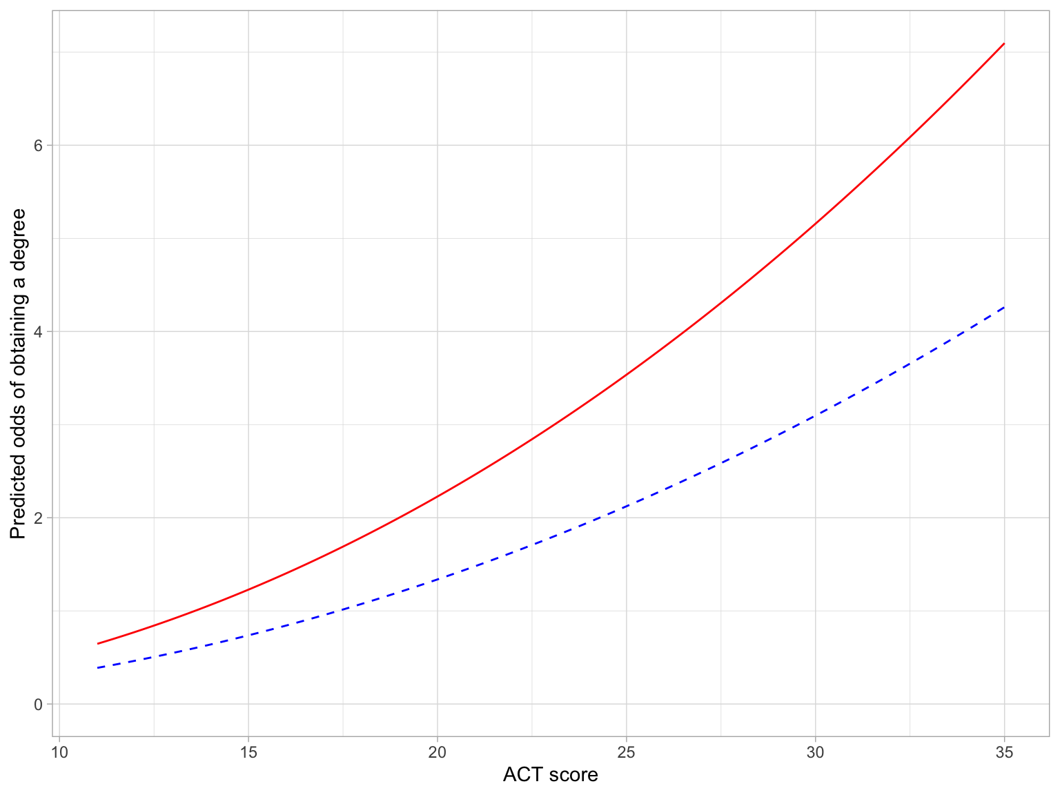
Here we see that the odds of graduating increase exponentially at higher ACT scores for both first generation and non-first generation students, on average. This rate of increase, however, is higher for first generation students. Moreover, first generation students have higher odds of graduating than non-first generation students, regardless of ACT score.
Back-Transforming to Probability
Again, while not related to the research question, we can also plot the predicted probability of graduating as a function of ACT score. Algebraically manipulating the fitted equation,
\[ \hat\pi_i = \frac{e^{-5.91 + 0.51(\mathrm{First~Generation}_i) + 2.07\bigg[\ln(\mathrm{ACT~Score}_i)\bigg]}}{1 + e^{-5.91 + 0.51(\mathrm{First~Generation}_i) + 2.07\bigg[\ln(\mathrm{ACT~Score}_i)\bigg]}} \]
We can then produce the fitted equations for non-first generation and first generation students by substituting either 0 or 1, respectively, into the firstgen variable. These equations are:
Non-First Generation Students
\[ \begin{split} \hat\pi_i &= \frac{e^{-5.91 + 0.51(0) + 2.07\bigg[\ln(\mathrm{ACT~Score}_i)\bigg]}}{1 + e^{-5.91 + 0.51(0) + 2.07\bigg[\ln(\mathrm{ACT~Score}_i)\bigg]}} \\[3ex] &= \frac{e^{-5.91 + 2.07\bigg[\ln(\mathrm{ACT~Score}_i)\bigg]}}{1 + e^{-5.91 + 2.07\bigg[\ln(\mathrm{ACT~Score}_i)\bigg]}} \end{split} \]
First Generation Students
\[ \begin{split} \hat\pi_i &= \frac{e^{-5.91 + 0.51(1) + 2.07\bigg[\ln(\mathrm{ACT~Score}_i)\bigg]}}{1 + e^{-5.91 + 0.51(1) + 2.07\bigg[\ln(\mathrm{ACT~Score}_i)\bigg]}} \\[1em] &= \frac{e^{-5.40 + 2.07\bigg[\ln(\mathrm{ACT~Score}_i)\bigg]}}{1 + e^{-5.40 + 2.07\bigg[\ln(\mathrm{ACT~Score}_i)\bigg]}} \end{split} \]
We can include each of these in a geom_function() layer in our plot.
# Plot the fitted equations
ggplot(data = grad, aes(x = act, y = got_degree)) +
  geom_point(alpha = 0) +
  # Non-first generation students
  geom_function(
    fun = function(x) {exp(-5.91 + 2.07*log(x)) / (1 + exp(-5.91 + 2.07*log(x)))},
    linetype = "dashed",
    color = "blue"
    ) +
  # First generation students
  geom_function(
    fun = function(x) {exp(-5.40 + 2.07*log(x)) / (1 + exp(-5.40 + 2.07*log(x)))},
    linetype = "solid",
    color = "red"
    ) +
  theme_light() +
  xlab("ACT score") +
  ylab("Predicted probability of obtaining a degree") +
  ylim(0, 1)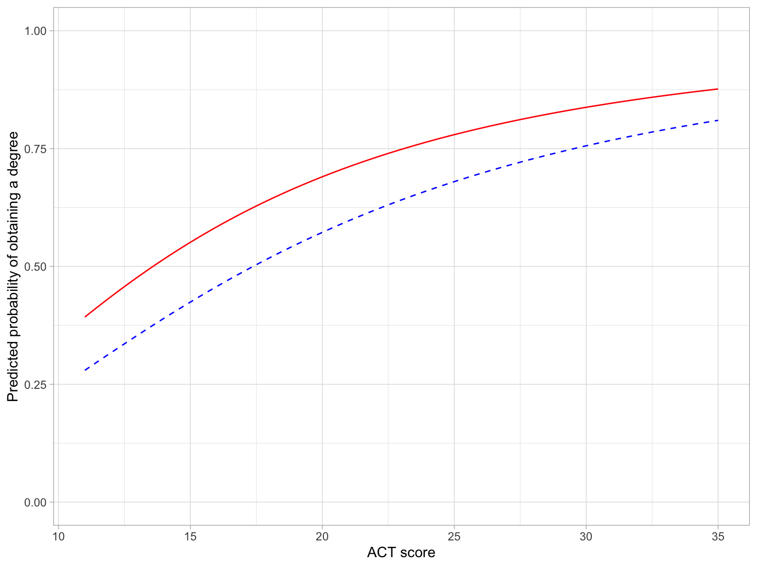
Here we see that the probability of graduatingobtaining a degree is positively associated with ACT score for both first generation and non-first generation students. The magnitude of the effect of ACT depends on ACT score for both groups. Although first generation students have higher probability of obtaining a degree than non-first generation students regardless of ACT score, the magnitude of this difference decreases at higher ACT scores.
Including Other Covariates in the Model
We will now fit a series of models that systematically include the remainder of the potential covariates based on their importance. We will have to adopt the correct functional form for ALL continuous variables by examining the plots of the data and residuals from potential transformations. (NOTE: This work is not shown here, but you should undertake it.)
The second covariate we will include is the number of AP courses taken. We use a log-transformation of this variable given its curvilinear status with the empirical log-odds of obtaining a degree. Because it has values of 0, we also add 1 before log-transforming.
# Log-linear effect of AP courses
glm.4 = glm(got_degree ~ 1 + is_firstgen + log(act) + log(ap_courses + 1), data = grad, family = binomial(link = "logit"))
Next, we include scholarship amount into the model. An examination of the empirical log-odds of obtaining a degree versus scholarship amount also suggested a curvilinear relationship. We adopt a log-linear model, again adding 1 prior to transforming using the logarithm since there are 0s in the variable.
# Effect of scholarship
glm.5 = glm(got_degree ~ 1 + is_firstgen + log(act) + log(ap_courses + 1) +  log(scholarship + 1), data = grad, family = binomial(link = "logit"))
Finally, we include the effect of non-traditional student status. Since it is a dummy-coded variable, we do not have to worry about the functional form. However, since we don’t know the functional form we need for scholarship amount, we will consider both when we include this covariate.
# Effect of non-traditional student
glm.6 = glm(got_degree ~ 1 + is_firstgen + log(act) + log(ap_courses + 1) + log(scholarship + 1) +
              is_nontrad, data = grad, family = binomial(link = "logit"))
Now we will use information criteria to select from these potential models.
aictab(
  cand.set = list(glm.2, glm.3, glm.4, glm.5, glm.6),
  modnames = c("FG", "FG + ACT", "FG + ACT + AP", "FG + ACT + AP + Sch",
               "FG + ACT + AP + Sch + NT")
)
Here the empirical evidence supports the model that includes all the covariates. Examining the binned residuals (not shown), the model does not seem adequate. Next we turn to evaluating potential interaction terms to see if that improves the residual fit.
Interaction Between ACT Score and First Generation Status
Since this is an exploratory analysis, we should only fit first-order interactions, and only with the focal predictor (i.e., first generation status). We will adopt the same modeling strategy as before, building up interaction terms in the order of covariate importance.
# Interaction models
glm.7 = glm(got_degree ~ 1 + is_firstgen + log(act) + log(ap_courses + 1) + log(scholarship + 1) +
              is_nontrad + is_firstgen:log(act), data = grad, family = binomial(link = "logit"))

glm.8 = glm(got_degree ~ 1 + is_firstgen + log(act) + log(ap_courses + 1) + log(scholarship + 1) +
              is_nontrad + is_firstgen:log(act) + is_firstgen:log(ap_courses + 1),
            data = grad, family = binomial(link = "logit"))

glm.9 = glm(got_degree ~ 1 + is_firstgen + log(act) + log(ap_courses + 1) + log(scholarship + 1) +
              is_nontrad + is_firstgen:log(act) + is_firstgen:log(ap_courses + 1) +
              is_firstgen:log(scholarship + 1),
            data = grad, family = binomial(link = "logit"))


glm.10 = glm(got_degree ~ 1 + is_firstgen + log(act) + log(ap_courses + 1) + log(scholarship + 1) +
              is_nontrad + is_firstgen:log(act) + is_firstgen:log(ap_courses + 1) +
              is_firstgen:log(scholarship + 1) + is_firstgen:is_nontrad,
            data = grad, family = binomial(link = "logit"))

# Evaluate
aictab(
  cand.set = list(glm.6, glm.7, glm.8, glm.9, glm.10),
  modnames = c("Main Effects", "FG:ACT", "FG:ACT + FG:AP", "FG:ACT + FG:APP + FG:Sch",
               "FG:ACT + FG:APP + FG:Sch + FG:NT")
)
While the model that includes the interaction between first generation status and ACT has the most empirical evidence (given the data and candidate models), there is some degree of empirical evidence for almost all of the interaction models fitted. Evaluating the binned residuals (not shown) there is a reasonable (and roughly equal) degree of residual fit for glm.7, glm.8, and glm.10. Given this, the information from the AICc table, and the rule of parsimony, we will adopt glm.7.
# Coefficients
tidy(glm.7)
\[ \begin{split} \ln\bigg[\frac{\hat\pi_i}{1 - \hat\pi_i}\bigg] = &-1.25 - 3.04(\mathrm{First~Gen}_i) + 0.54\bigg[\ln(\mathrm{ACT~Score}_i)\bigg] + 0.28\bigg[\ln(\mathrm{AP~Courses}_i + 1)\bigg] +\\ & 1.11\bigg[\ln(\mathrm{Scholarship}_i + 1)\bigg] - 0.83(\mathrm{Non\mbox{-}Traditional}_i) + 1.10\bigg[\ln(\mathrm{ACT~Score}_i\bigg](\mathrm{First~Gen}_i) \end{split} \]
Interpreting the Results from the Adopted Model
To interpret these results, we will plot results freom the fitted model. In thinking about what needs to be displayed:
- The effect of first-generation student wil be displayed as separate lines since it is the focal predictor.
- The effect of ACT will be displayed since it is part of an interaction with the focal predictor.
- The effect of AP Courses will be controlled out by setting to its mean value.
- The effect of Scholarship will be controlled out by setting to its mean value.
- The effect of Non-traditional will be controlled by setting the value to the reference level (e.g., traditional student).1
We next use the fitted equation to find the equations for the first and non-first generation students.
Non-First Generation Students
\[ \begin{split} \ln\bigg[\frac{\hat\pi_i}{1 - \hat\pi_i}\bigg] = &-1.25 - 3.04(0) + 0.54\bigg[\ln(\mathrm{ACT~Score}_i)\bigg] + 0.28\bigg[\ln(3.28 + 1)\bigg] +\\ & 1.11\bigg[\ln(0.18 + 1)\bigg] - 0.83(0) + 1.10\bigg[\ln(\mathrm{ACT~Score}_i\bigg](0) \\[3ex] = & -0.66 + 0.54\bigg[\ln(\mathrm{ACT~Score}_i)\bigg] \end{split} \]
First Generation Students
\[ \begin{split} \ln\bigg[\frac{\hat\pi_i}{1 - \hat\pi_i}\bigg] = &-1.25 - 3.04(1) + 0.54\bigg[\ln(\mathrm{ACT~Score}_i)\bigg] + 0.28\bigg[\ln(3.28 + 1)\bigg] +\\ & 1.11\bigg[\ln(0.18 + 1)\bigg] - 0.83(0) + 1.10\bigg[\ln(\mathrm{ACT~Score}_i\bigg](1) \\[3ex] = & -3.70 + 1.64\bigg[\ln(\mathrm{ACT~Score}_i)\bigg] \end{split} \]
We will plot these two equations using the probability metric.
# Plot the fitted equations
ggplot(data = grad, aes(x = act, y = got_degree)) +
  geom_point(alpha = 0) +
  # Non-first generation students
  geom_function(
    fun = function(x) {exp(-0.66 + 0.54*log(x)) / (1 + exp(-0.66 + 0.5*log(x)))},
    linetype = "dashed",
    color = "blue"
    ) +
  # First generation students
  geom_function(
    fun = function(x) {exp(-3.70 + 1.64*log(x)) / (1 + exp(-3.70 + 1.647*log(x)))},
    linetype = "solid",
    color = "red"
    ) +
  theme_light() +
  xlab("ACT score") +
  ylab("Predicted probability of obtaining a degree") +
  ylim(0, 1)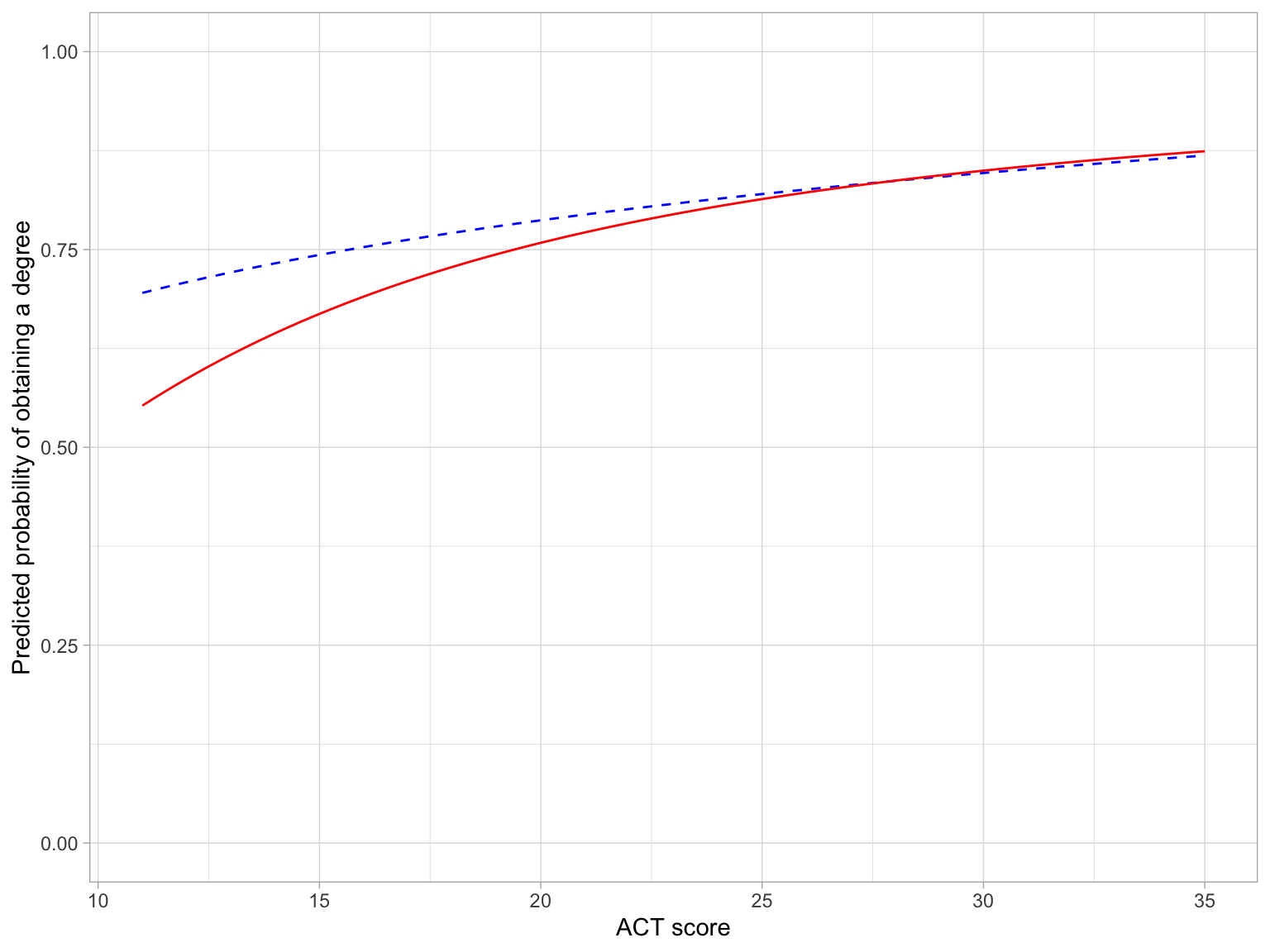
Because our research question is about the effect of first generation status, we will focus the interpretation from this plot on that effect.
Here we see that first generation status and ACT score interact on the probability of obtaining a degree. For students with lower ACT scores the probability of obtaining a degree is smaller for first generation students than for non-first generation students. However, this difference diminishes for students with higher ACT scores.
Presenting a Table of Logistic Regression Results
We can present selected fitted models from the analysis in a table similar to those we have created for OLS models. In this analysis I would present glm.0, glm.2, glm.3, glm.6, and glm.7. Note that we do not have to present ALL the models we fitted in the table, only those that tell a coherent story about the analysis. (If you are worried about transparency, you can always link to our script file or RMD document which includes all the models fitted in the paper, or include some prose that indicates there were other models fitted.) For these models, we want to report:
- Coefficients and SEs
- Residual Deviance
- AICc values (This can be computed from the df and residual deviances, but since it was our main criterion for model selection, it is a good idea to report it!)
- Pseudo-\(R^2\) values
Here is a table I might present for this analysis.
Code
# Create the table
htmlreg(
  l = list(glm.0, glm.2, glm.3, glm.6, glm.7),
  stars = numeric(0),    #No p-value stars
  digits = 2,
  padding = 20,          #Add space around columns (you may need to adjust this via trial-and-error)
  custom.model.names = c("Model A", "Model B", "Model C", "Model D", "Model E"),
  custom.coef.names = c("Intercept", "First Generation", "ln(ACT Score)",
                        "ln(AP Courses + 1)", "ln(Scholarship Amount + 1)", "Non-Traditional Student",
                        "First Generation x ln(ACT Score)"),
  reorder.coef = c(2:7, 1), #Put intercept at bottom of table
  include.aic = FALSE, #Omit AIC
  include.bic = FALSE, #Omit BIC
  include.nobs = FALSE,  #Omit sample size
  include.loglik = FALSE,   #Omit log-likelihood
  custom.gof.rows = list(
    AICc = c(AICc(glm.0), AICc(glm.2), AICc(glm.3), AICc(glm.6), AICc(glm.7)),
    R2 = (2722.5 - c(NA, 2662.09, 2605.00, 2540.35, 2536.67)) /  2722.5
    ), # Add AICc values
  reorder.gof = c(3, 1, 2),
  caption = NULL,
  caption.above = TRUE, #Move caption above table
  inner.rules = 1, #Include line rule before model-level output
  outer.rules = 1 , #Include line rules around table
  custom.note = "The $R^2$ value is based on the proportion of reduced deviance from the intercept-only model (Model A)"
  )
Five candidate models predicting variation in the log-odds of obtaining a degree. The first generation and non-traditional student predictors were dummy-coded.
|
|
Model A
|
Model B
|
Model C
|
Model D
|
Model E
|
|---|---|---|---|---|---|
|
First Generation
|
|
0.77
|
0.51
|
0.42
|
-3.04
|
|
|
|
(0.10)
|
(0.10)
|
(0.11)
|
(1.80)
|
|
ln(ACT Score)
|
|
|
2.07
|
1.11
|
0.54
|
|
|
|
|
(0.28)
|
(0.30)
|
(0.42)
|
|
ln(AP Courses + 1)
|
|
|
|
0.29
|
0.28
|
|
|
|
|
|
(0.06)
|
(0.06)
|
|
ln(Scholarship Amount + 1)
|
|
|
|
1.16
|
1.11
|
|
|
|
|
|
(0.26)
|
(0.26)
|
|
Non-Traditional Student
|
|
|
|
-0.84
|
-0.83
|
|
|
|
|
|
(0.33)
|
(0.33)
|
|
First Generation x ln(ACT Score)
|
|
|
|
|
1.10
|
|
|
|
|
|
|
(0.57)
|
|
Intercept
|
1.01
|
0.50
|
-5.91
|
-3.03
|
-1.25
|
|
|
(0.05)
|
(0.08)
|
(0.86)
|
(0.94)
|
(1.31)
|
|
Deviance
|
2722.55
|
2662.09
|
2605.00
|
2540.35
|
2536.67
|
|
AICc
|
2724.55
|
2666.09
|
2611.01
|
2552.39
|
2550.72
|
|
R2
|
|
0.02
|
0.04
|
0.07
|
0.07
|
|
The \(R^2\) value is based on the proportion of reduced deviance from the intercept-only model (Model A)
|
|||||
Pseudo-\(R^2\) values are commonly reported in applied research. Because there are many potential pseudo-\(R^2\) values, you should always indicate the method used to calculate this metric.
Footnotes
Another analyst might choose to use the non-traditional group or to show the effect by displaying both groups, perhaps in different panels.↩︎