Graphical Evaluation of Residuals

Andrew Zieffler

7/14/2022

The educate package includes the residual_plots() function to generate plots of the standardized residuals along with confidence envelopes to help evaluate model assumptions. Below I illustrate the usage of this function.

Evaluate Normality

# Load libraries
library(broom)
library(ggplot2)
library(educate)

# Fit a linear model
lm.1 = lm(speed ~ dist, data = cars)

# Density plot
residual_plots(lm.1, type = "d")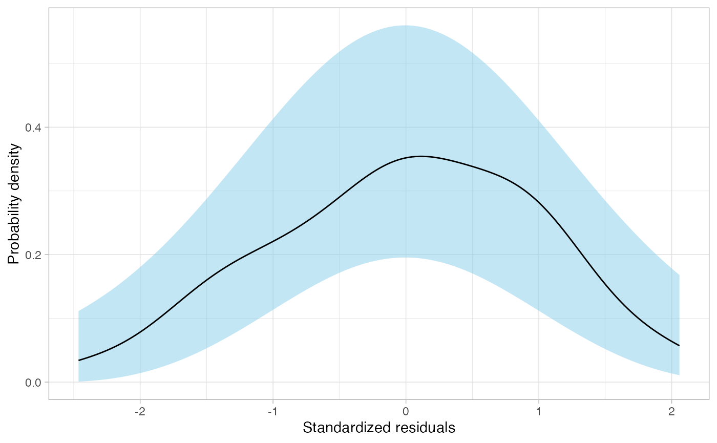

You need to provide the fitted model object (in the model= argument; typically unnamed). You also need to provide the plot type using the type= argument. Here we use type="d" to obtain the density plot of the standardized residuals.

Evaluate Linearity and Homoskedasticity

# Load libraries
library(broom)
library(ggplot2)
library(educate)

# Fit a linear model
lm.1 = lm(speed ~ dist, data = cars)

# Density plot
residual_plots(lm.1, type = "s")

## `geom_smooth()` using formula = 'y ~ x'
## `geom_smooth()` using formula = 'y ~ x'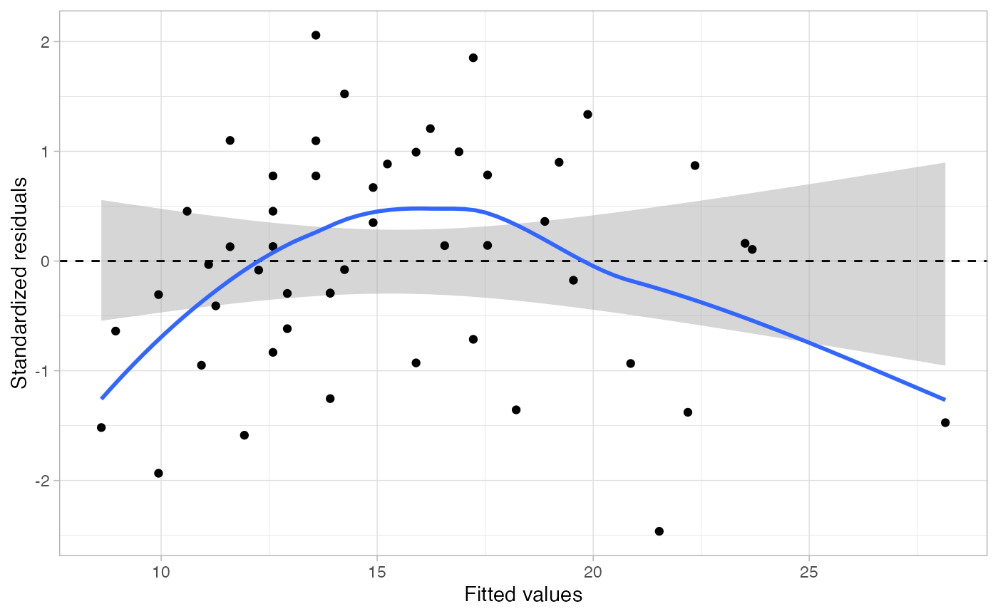

Here we use type="s" to obtain the the scatterplot of the standardized residuals versus the fitted values.

Both Residual Plots

# Load libraries
library(broom)
library(ggplot2)
library(educate)
library(patchwork)

# Fit a linear model
lm.1 = lm(speed ~ dist, data = cars)

# Both residual plots
residual_plots(lm.1, type = "b")

## `geom_smooth()` using formula = 'y ~ x'
## `geom_smooth()` using formula = 'y ~ x'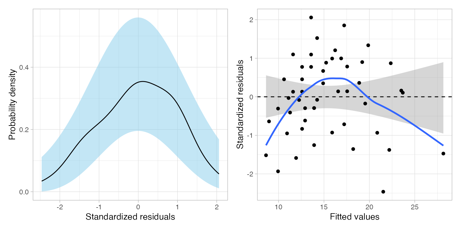

# residual_plots(lm.1)

To obtain both plots requires that the patchwork package is loaded. Here we use type="b" to obtain both the density plot of the standardized residuals, and the scatterplot of the standardized residuals versus the fitted values. You can also omit the type= argument, since the default is type="b".