LMER: Other Random-Effects and Covariates
In this set of notes, you will continue to learn how to use the linear mixed-effects model to examine the mean change over time in a set of longitudinal/repeated measurements. You will also learn how to expand the model to allow cases to have different growth rates. Lastly, you will learn how to include covariates to evaluate whether the average growth rates vary for different groups. To do so, we will use data from the file minneapolis.csv.
We will use these data to explore the change in students’ reading scores over time (i.e., is there longitudinal variation in students’ reading scores). As in most longitudinal analyses, our primary goal is to examine the mean change (i.e., pattern of growth) of the outcome over time.
# Load libraries
library(AICcmodavg)
library(broom.mixed) #for tidy, glance, and augment functions for lme4 models
library(corrr)
library(educate)
library(lme4) #for fitting mixed-effects models
library(patchwork)
library(texreg)
library(tidyverse)

# Import data
mpls = read_csv("https://raw.githubusercontent.com/zief0002/bespectacled-antelope/main/data/minneapolis.csv")

# View data
mpls
The data are already in the long/tidy format, so we do not need to re-structure them. We will start the analysis by examining the average and individual growth profiles.
ggplot(data = mpls, aes(x = grade, y = reading_score)) +
  geom_line(aes(group = student_id), alpha = 0.3) +  #Add individual profiles
  stat_summary(fun = mean, geom = "line", size = 2, group = 1, color = "#FF2D21") + #Add mean profile line
  theme_light() +
  xlab("Grade") +
  ylab("Reading Score")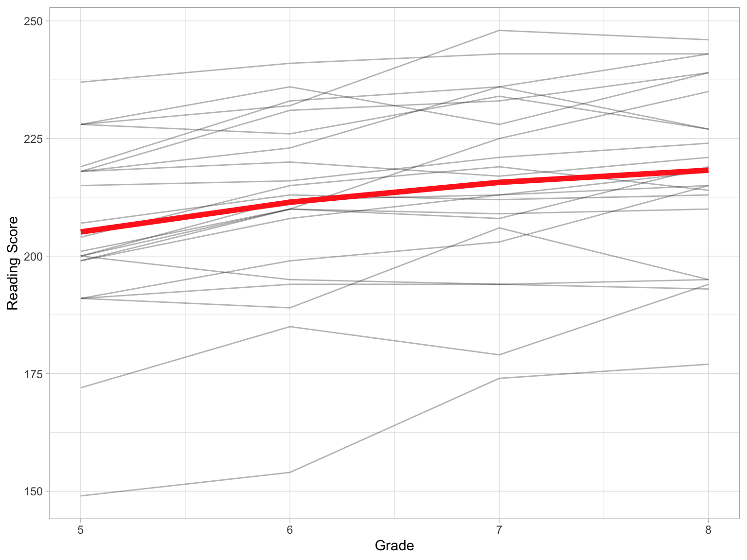
Focusing on the average growth profile, it appears that the students’ average reading score gets higher over time, and that this change is fairly linear. We will next fit the unconditional random intercepts model (to get a baseline measure of the unaccounted for variation) and the unconditional linear growth model. In the latter model we center grade on the initial measurement occasion. We display the results from these fitted models in a table.
# Fit unconditional random-intercepts models
lmer.a = lmer(reading_score ~ 1 + (1 | student_id), data = mpls, REML = FALSE)

#Fit unconditional growth model with centered grade
lmer.b = lmer(reading_score ~ 1 + I(grade-5) + (1 | student_id), data = mpls, REML = FALSE)

# Coefficient-level output (not displayed)
# tidy(lmer.a, effects = "fixed")
# tidy(lmer.b, effects = "fixed")

# Variance estimates (not displayed)
# tidy(lmer.a, effects = "ran_pars")
# tidy(lmer.b, effects = "ran_pars")
Code
htmlreg(
  l = list(lmer.a, lmer.b),
  stars = numeric(0),    #No p-value stars
  digits = 2,
  padding = 20, #Add space around columns (you may need to adjust this via trial-and-error)
  custom.model.names = c("Model A", "Model B"),
  custom.coef.names = c("Intercept", "Grade"),
  reorder.coef = c(2, 1), #Put intercept at bottom of table
  include.loglik = FALSE, #Omit log-likelihood
  include.aic = FALSE,    #Omit AIC
  include.bic = FALSE,    #Omit BIC
  include.nobs = FALSE,   #Omit sample size
  include.groups = FALSE, #Omit group size
  include.deviance = TRUE,
  custom.gof.names = c("Deviance", "Level-2 Variance (Intercept)", "Level-1 Variance"), # Rename variance component rows
  custom.gof.rows = list(
    AICc = c(AICc(lmer.a), AICc(lmer.b))  # Add AICc values
  ),
  reorder.gof = c(3, 4, 2, 1),
  caption = NULL,
  caption.above = TRUE, #Move caption above table
  inner.rules = 1, #Include line rule before model-level output
  outer.rules = 1 , #Include line rules around table
  custom.note = "*Note.* The grade predictor was centered at the initial measurement occasion of 5th-grade."
)| Model A | Model B | |
|---|---|---|
| Grade | 4.36 | |
| (0.52) | ||
| Intercept | 212.64 | 206.09 |
| (3.96) | (4.04) | |
| Level-2 Variance (Intercept) | 329.66 | 337.57 |
| Level-1 Variance | 61.62 | 29.89 |
| Deviance | 680.78 | 633.02 |
| AICc | 687.07 | 641.50 |
| Note. The grade predictor was centered at the initial measurement occasion of 5th-grade. | ||
Taxonomy of models predicting longitudinal variation in students' reading scores.
From Model A we find that most of the unaccounted for variation in reading scores is between-student variation (84%). There is also unaccounted for variation at the within-student level. Model B includes the time-varying predictor of grade to explain within-student variation. This model explains 51.4% of the within-student variation, and \(-2.2\)% of the between-student variation (mathematical artifact). Below we write the global fitted equation and Student 1 and 2’s fitted equation based on the results of Model B.
\[ \begin{split} \mathbf{Global:~} \hat{\mathrm{Reading~Score}}_{ij} &= 206 + 4.36(\mathrm{Grade}_{ij} - 5) \\[1ex] \mathbf{Student~1:~} \hat{\mathrm{Reading~Score}}_{i1} &= 177 + 4.36(\mathrm{Grade}_{i1} - 5) \\[1ex] \mathbf{Student~2:~} \hat{\mathrm{Reading~Score}}_{i2} &= 201 + 4.36(\mathrm{Grade}_{i2}-5 ) \\[1ex] \end{split} \]
The coefficient interpretations from the global fitted equation are:
- The predicted average reading score for all students at the initial measurement occasion (in the 5th grade) is 206.
- Each subsequent grade-level is associated with a 4.36-point change in reading score, on average.
The unconditional growth model we fitted included a random-effect of intercept. This term accounted for the non-independence of reading scores in the data. It also allowed the student-specific equations to differ from the global equation in the intercept. That is, it allowed students to have different reading scores at the initial measurement occasion. Substantively, this implies that the reason an individual student has a higher (or lower) reading score than average is because their reading score at the initial measurement occasion was higher (or lower) than the average student.
Another reason that students might have a higher (or lower) reading score than average is because their growth rate is different than the average growth rate. The model we fitted did not allow students to have different growth rates than the average student. To evaluate whether we should allow this kind of flexibility in the model, we will focus on a plot of the individual student profiles to see whether they appear to have different rates-of-growth than the average profile.
Plots of the Individual Student Profiles
Although we included the student profiles in the spaghetti plot we created earlier, in cases with a larger number of students it would be difficult to see the individual profiles in the spaghetti plot. To remedy this, you could facet on student so that each individual profile appears in a separate panel of the plot. (Note: If you have a lot of cases, rather than looking at all profiles, you could select a random sample of the cases and view those profiles.)
# Get the mean reading score at each grade
# Need to use this to add the average profile in each facet
global = mpls |>
  group_by(grade) |>
  summarize(
    reading_score = mean(reading_score)
    ) |>
  ungroup()

# Plot individual profiles in different panels
# Add average profile to each panel
ggplot(data = mpls, aes(x = grade, y = reading_score)) +
  geom_line(aes(group = student_id), alpha = 0.3) + #Individual profiles
  geom_line(data = global, size = 2, group = 1, color = "#FF2D21") + #Mean profile
  theme_light() +
  xlab("Grade") +
  ylab("Reading Score")  +
  facet_wrap(~student_id)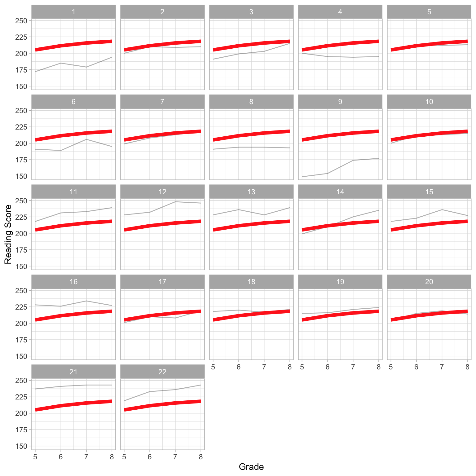
The different slopes seen in the individual profiles indicate that students have different growth rates in their reading score over time, which also differ from the average growth rate. For example, Students 14 and 22 have higher growth rates than the average student. Student 16, on the other hand, has a smaller growth rate than the average student. This suggests that we also need to include a random-effect of grade (time) in our model.
Unconditional Growth Model with Random-Effects of Intercept and Grade-Level
The statistical model that includes random-effects for intercepts and grade-level can be expressed as:
\[ \mathrm{Reading~Score}_{ij} = \big[\beta_0 + b_{0j}\big] + \big[\beta_1 + b_{1j}\big](\mathrm{Grade}_{ij}-5) + \epsilon_{ij} \]
where,
- \(\mathrm{Reading~Score}_{ij}\) is the reading score for Student j at time point i;
- \(\beta_0\) is the fixed-effect of intercept;
- \(b_{0j}\) is the random-effect of intercept for Student j;
- \(\beta_1\) is the fixed-effect of grade-level;
- \(b_{1j}\) is the random-effect of grade-level for Student j; and
- \(\epsilon_{ij}\) is the error for Student j at time point i.
We fit the model and display the output below. We it the model using ML estimation.
# Fit model
lmer.c = lmer(reading_score ~ 1 + I(grade-5) + (1 + I(grade-5) | student_id), data = mpls, REML = FALSE)

# Coefficient-level output
tidy(lmer.c, effects = "fixed")
Using the fixed-effects estimates, the global fitted equation based on the fixed-effects model is:
\[ \hat{\mathrm{Reading~Score}_{ij}} = 206 + 4.36(\mathrm{Grade}_{ij}-5) \]
The coefficient interpretations are:
- The predicted average reading score for all students at the initial measurement occasion (in the 5th grade) is 206.
- Each subsequent grade-level is associated with a 4.36-point change in reading score, on average.
The fixed-effects did not change much as a result of allowing individual students to have different growth rates. We can also write the student specific fitted equations. Each student specific fitted equation is based on the fixed-effects AND the student-specific random-effects.
# Obtain random effects
tidy(lmer.c, effects = "ran_vals")
# Obtain random effects for Student 1
tidy(lmer.c, effects = "ran_vals") |>
filter(level == 1)For example, Student 1’s fitted equation is:
\[ \begin{split} \hat{\mathrm{Reading~Score}_{i1}} &= \bigg[206 - 31.8\bigg] + \bigg[4.36 + 1.33\bigg](\mathrm{Grade}_{i1}-5) \\[1ex] &= 174.2 + 5.69(\mathrm{Grade}_{i1}-5) \\[1ex] \end{split} \]
- The predicted reading score for Student 1 at the initial measurement occasion is 174.2 (31.8 points lower than the average student at that grade).
- For Student 1, each subsequent grade is associated with a 5.69-point change in reading score, on average (a growth rate that is 1.33 points per grade higher than average).
Recall the argument effects="ran_coefs" in the tidy() function gives the student-specific effects directly.
# Obtain student-specific coefficients for Student 2
tidy(lmer.c, effects = "ran_coefs") |>
  filter(level == 2)
From here, we see that Student 2’s fitted equation is:
\[ \hat{\mathrm{Reading~Score}_{i2}} = 202 + 3.42(\mathrm{Grade}_{i2}-5) \]
From the two students’ fitted equations we see that by including a random-effect of both intercept and grade (time):
- Students can have a different reading score than average at the initial measurement occasion.
- Students can have a different growth rate than the average growth rate.
Variance Estimates
We can also examine the variance components for the fitted model:
# Obtain variance estimates
tidy(lmer.c, effects = "ran_pars")
We now have four total variance components:
- Between-Student Variance (Intercept): \(\mathrm{Var}(b_0) = 19.5^2 = 380.25\)
- Between-Student Variance (Rate-of-Change): \(\mathrm{Var}(b_1) = 2.72^2 = 7.40\)
- Between-Student Correlation (between Intercepts and Rate-of-Change): \(\mathrm{Corr}(b_0,b_1) = -0.36\)
- Within-Student Variance: \(\mathrm{Var}(e) = 4.19^2 = 17.56\)
Between-student variance components are Level-2 variance components and the within-student variance component is the Level-1 variance component.
Adding a random-effect resulted in two additional variance components. We now have split the between-student variance into two parts: (1) variation in students’ intercepts, and (2) variation in students growth rates. That is we are saying that variation in reading scores is due to student differences in reading scores at the initial measurement occasion, differences in students’ growth rates, and within-student variation (random error).
The correlation indicates the relationship between the student-specific random effects of intercept and rate-of-change. The fact that this is negative indicates that students who have a lower random-effect of intercept tend to have a higher random-effect of grade In other words, students who have a lower reading score at the initial measurement occasion tend to have a higher growth rate.
Below, we add Model C to our table of regression results.
Code
htmlreg(
  l = list(lmer.a, lmer.b, lmer.c),
  stars = numeric(0),    #No p-value stars
  digits = 2,
  padding = 20, #Add space around columns (you may need to adjust this via trial-and-error)
  custom.model.names = c("Model A", "Model B", "Model C"),
  custom.coef.names = c("Intercept", "Grade"),
  reorder.coef = c(2, 1), #Put intercept at bottom of table
  include.loglik = FALSE, #Omit log-likelihood
  include.aic = FALSE,    #Omit AIC
  include.bic = FALSE,    #Omit BIC
  include.nobs = FALSE,   #Omit sample size
  include.groups = FALSE, #Omit group size
  include.deviance = TRUE,
  custom.gof.names = c("Deviance", "Level-2 Variance (Intercept)", "Level-1 Variance", "Level-2 Variance (Slope)", "Level-2 Covariance"), # Rename variance component rows
  custom.gof.rows = list(
    AICc = c(AICc(lmer.a), AICc(lmer.b), AICc(lmer.c))  # Add AICc values
  ),
  reorder.gof = c(3, 5, 6, 4, 2, 1),
  caption = NULL,
  caption.above = TRUE, #Move caption above table
  inner.rules = 1, #Include line rule before model-level output
  outer.rules = 1 , #Include line rules around table
  custom.note = "*Note.* The grade predictor was centered at the initial measurement occasion of 5th-grade."
)| Model A | Model B | Model C | |
|---|---|---|---|
| Grade | 4.36 | 4.36 | |
| (0.52) | (0.70) | ||
| Intercept | 212.64 | 206.09 | 206.09 |
| (3.96) | (4.04) | (4.23) | |
| Level-2 Variance (Intercept) | 329.66 | 337.57 | 381.44 |
| Level-2 Variance (Slope) | 7.38 | ||
| Level-2 Covariance | -19.12 | ||
| Level-1 Variance | 61.62 | 29.89 | 17.59 |
| Deviance | 680.78 | 633.02 | 622.52 |
| AICc | 687.07 | 641.50 | 635.56 |
| Note. The grade predictor was centered at the initial measurement occasion of 5th-grade. | |||
Taxonomy of models predicting longitudinal variation in students' reading scores.
Notice that the htmlreg() function produces the covariance between the intercept and slope random effects rather than the correlation that is produced from tidy(). There is a direct relationship between the correlation and covariance:
\[ \mathrm{Cov}(b_0,b_1) = \mathrm{Corr}(b_0,b_1) \times \sqrt{\mathrm{Var}(b_0)} \times \sqrt{\mathrm{Var}(b_1)} \]
In our example,
\[ \begin{split} \mathrm{Cov}(b_0,b_1) &= -0.360 \times \sqrt{380.25} \times \sqrt{7.3984} \\[1ex] &= -19.09 \end{split} \] Sometimes the variances and covariances of the random-effects are reported in a matrix referred to as the variance-covariance matrix of random-effects and denoted as G.
\[ \mathbf{G} = \begin{bmatrix}\mathrm{Var}(b_0) & \mathrm{Cov}(b_0,b_1)\\ \mathrm{Cov}(b_0,b_1) & \mathrm{Var}(b_1)\end{bmatrix} \]
In our example,
\[ \mathbf{G} = \begin{bmatrix}380.25 & -19.09\\ -19.09 & 7.40\end{bmatrix} \]
Explained Variation and Pseudo-\(R^2\) Values
It is difficult to compare the variance components for Model C to those from the unconditional random intercepts model to get pseudo-\(R^2\) values, like we did for Model B. This is because Model C includes an additional source of unexplained variation, namely \(Var(b_1)\) that the unconditional random intercepts model did not include.
As we add other fixed-effects predictors to the model, the variance components from those models could be compared to the variance components from Model C (so long as these models continue to include both the random intercepts and slopes). In other words, Model C becomes the new baseline model for other models that also include random intercepts and slopes.
Group Differences in the Average Growth Profiles
One question we might have is whether the average growth profile varies across different groups. For example, we might wonder if (and how) the average growth profile is different for special education and non-special education students. To explore this, we will again create a spaghetti plot, but this time we will facet on special education status.
ggplot(data = mpls, aes(x = grade, y = reading_score)) +
  geom_line(aes(group = student_id), alpha = 0.3) +  #Add individual profiles
  stat_summary(fun = mean, geom = "line", size = 2, group = 1, color = "#FF2D21") + #Add mean profile line
  theme_light() +
  xlab("Grade") +
  ylab("Reading Score") +
  facet_wrap(~special_ed)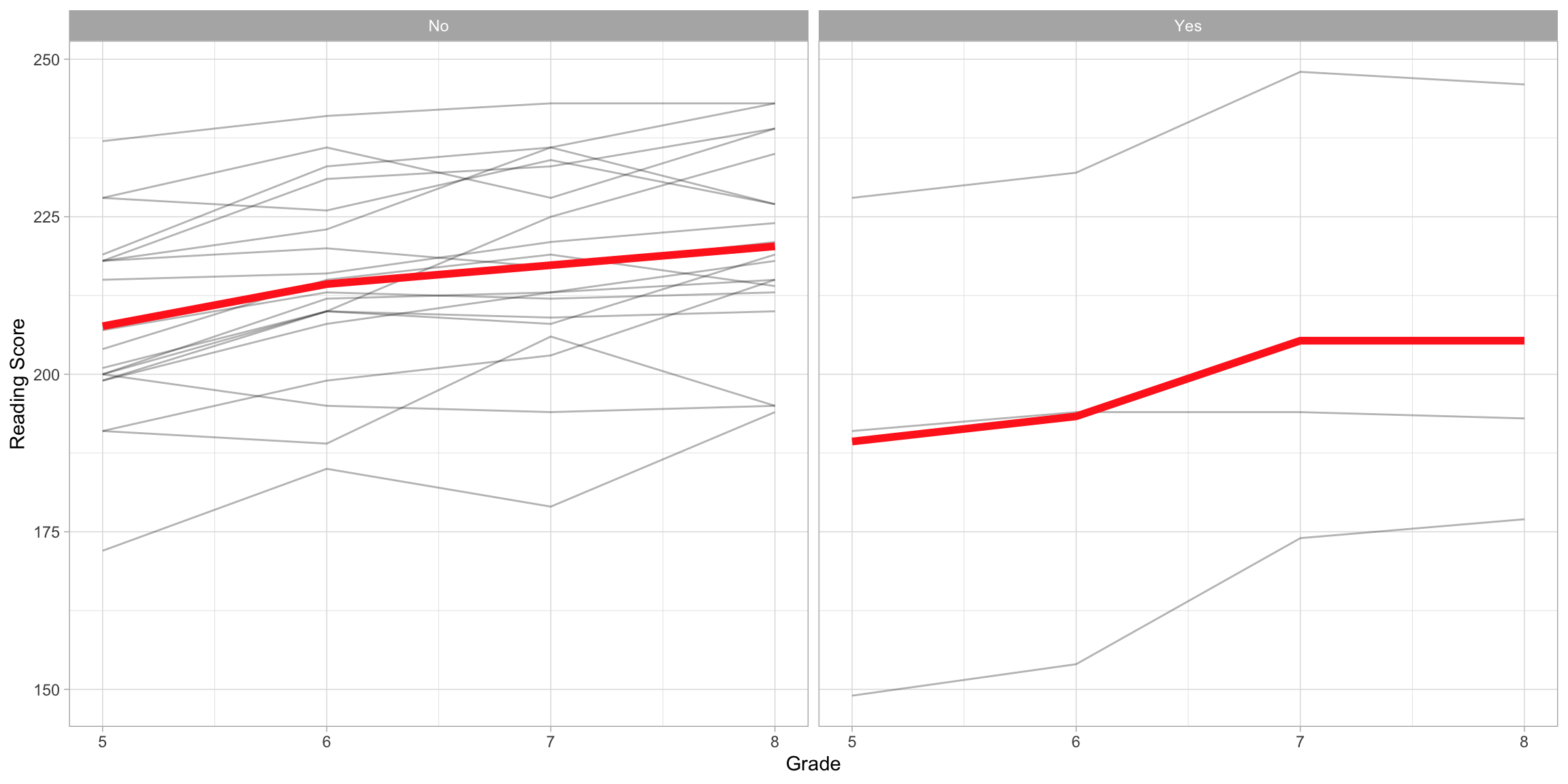
From this plot we see that the average profiles are different depending on special education status. To evaluate whether these differences are due to more than just sampling variation, we will fit a mixed-effects model that includes special education status as a fixed-effect. The statistical model that includes random-effects for intercepts and grade-level can be expressed as:
\[ \mathrm{Reading~Score}_{ij} = \big[\beta_0 + b_{0j}\big] + \big[\beta_1 + b_{1j}\big](\mathrm{Grade}_{ij}-5) + \beta_2(\mathrm{Special~Education}_j) + \epsilon_{ij} \]
where,
- \(\mathrm{Reading~Score}_{ij}\) is the reading score for Student j at time point i;
- \(\beta_0\) is the fixed-effect of intercept;
- \(b_{0j}\) is the random-effect of intercept for Student j;
- \(\beta_1\) is the fixed-effect of grade-level;
- \(b_{1j}\) is the random-effect of grade-level for Student j;
- \(\beta_2\) is the fixed-effect of special education status; and
- \(\epsilon_{ij}\) is the error for Student j at time point i.
Notice that th special education predictor only includes a j subscript. That is because it only varies between students. In our data, a single student has the same special education status at every time point. Therefore we do not put an i subscript on this predictor. We fit the model and display the output below. We again fit the model using ML estimation. We obtain both the fixed-effect estimates and estimated variance components for the fitted model and add these results to our table of regression results.
# Create dummy-coded special education status
mpls = mpls |>
  mutate(
    sped = if_else(special_ed == "Yes", 1, 0)
    )

# Fit model
lmer.d = lmer(reading_score ~ 1 + I(grade-5) + sped + (1 + I(grade-5) | student_id), data = mpls, REML = FALSE)

# Coefficient-level output
tidy(lmer.d, effects = "fixed")
# Obtain variance estimates
tidy(lmer.d, effects = "ran_pars")Code
htmlreg(
  l = list(lmer.a, lmer.b, lmer.c, lmer.d),
  stars = numeric(0),    #No p-value stars
  digits = 2,
  padding = 20, #Add space around columns (you may need to adjust this via trial-and-error)
  custom.model.names = c("Model A", "Model B", "Model C", "Model D"),
  custom.coef.names = c("Intercept", "Grade", "Special Education Status"),
  reorder.coef = c(2, 3, 1), #Put intercept at bottom of table
  include.loglik = FALSE, #Omit log-likelihood
  include.aic = FALSE,    #Omit AIC
  include.bic = FALSE,    #Omit BIC
  include.nobs = FALSE,   #Omit sample size
  include.groups = FALSE, #Omit group size
  include.deviance = TRUE,
  custom.gof.names = c("Deviance", "Level-2 Variance (Intercept)", "Level-1 Variance", "Level-2 Variance (Slope)", "Level-2 Covariance"), # Rename variance component rows
  custom.gof.rows = list(
    AICc = c(AICc(lmer.a), AICc(lmer.b), AICc(lmer.c), AICc(lmer.d))  # Add AICc values
  ),
  reorder.gof = c(3, 5, 6, 4, 2, 1),
  caption = NULL,
  caption.above = TRUE, #Move caption above table
  inner.rules = 1, #Include line rule before model-level output
  outer.rules = 1 , #Include line rules around table
  custom.note = "*Note.* The grade predictor was centered at the initial measurement occasion of 5th-grade. Special education status was dummy-coded using non-special education students as the reference group."
)| Model A | Model B | Model C | Model D | |
|---|---|---|---|---|
| Grade | 4.36 | 4.36 | 4.36 | |
| (0.52) | (0.70) | (0.70) | ||
| Special Education Status | -15.77 | |||
| (10.96) | ||||
| Intercept | 212.64 | 206.09 | 206.09 | 208.24 |
| (3.96) | (4.04) | (4.23) | (4.26) | |
| Level-2 Variance (Intercept) | 329.66 | 337.57 | 381.44 | 338.62 |
| Level-2 Variance (Slope) | 7.38 | 7.38 | ||
| Level-2 Covariance | -19.12 | -15.60 | ||
| Level-1 Variance | 61.62 | 29.89 | 17.59 | 17.59 |
| Deviance | 680.78 | 633.02 | 622.52 | 620.61 |
| AICc | 687.07 | 641.50 | 635.56 | 636.01 |
| Note. The grade predictor was centered at the initial measurement occasion of 5th-grade. Special education status was dummy-coded using non-special education students as the reference group. | ||||
Taxonomy of models predicting longitudinal variation in students' reading scores.
Using the fixed-effects estimates, the global fitted equation based on the fixed-effects model is:
\[ \hat{\mathrm{Reading~Score}_{ij}} = 208 + 4.36(\mathrm{Grade}_{ij}-5) - 15.8(\mathrm{Special~Education}_j) \]
The coefficient interpretations are:
- The predicted average reading score for non-special education students at the initial measurement occasion (in the 5th grade) is 208.
- Each subsequent grade-level is associated with a 4.36-point change in reading score, on average, controlling for special education status.
- Special education students have a reading score that is 15.8 points lower than non-special education students, on average, at every grade level.
We again have four total variance components:
- Between-Student Variance (Intercept): \(\mathrm{Var}(b_0) = 18.4^2 = 338.56\)
- Between-Student Variance (Rate-of-Change): \(\mathrm{Var}(b_1) = 2.72^2 = 7.40\)
- Between-Student Correlation (between Intercepts and Rate-of-Change): \(\mathrm{Corr}(b_0,b_1) = -0.312\)
- Within-Student Variance: \(\mathrm{Var}(e) = 4.19^2 = 17.56\)
Since this model includes the same set of random effects as Model C (unconditional growth model), we can use Model C as a baseline to consider the variation explained by special education status. Here we compute pseudo-\(R^2\) values based on using Model C as the comparison model.
- Between-Student Variance (Intercept): \((380.25 - 338.56)/380.25 = 0.110\)
- Between-Student Variance (Rate-of-Change): \((7.40 - 7.40)/7.40 = 0\)
- Within-Student Variance: \((17.56 - 17.56)/17.56=0\)
Including special education status explained 11% of the between-student variation in intercepts. This means it is helping to explain why students reading scores are different at the initial measurement occasion. It does not explain variation in students’ growth rates, nor does it explain within-student variation.
Student-Specific Fitted Equations
We again need to obtain the estimated random-effects for students in order to write their fitted equations. Moreover, we will also need their special education status. For example, we obtain Student 1’s random-effects using:
# Obtain student-specific coefficients for Student 2
tidy(lmer.d, effects = "ran_vals") |>
  filter(level == 1)
We also note that Student 1 is a non-special education student. Writing this student’s fitted equation:
\[ \begin{split} \hat{\mathrm{Reading~Score}_{i1}} &= \bigg[208 -33.7\bigg] + \bigg[4.36 + 1.26\bigg](\mathrm{Grade}_{i1}-5) - 15.77(0) \\[1ex] &= 174.3 + 5.62(\mathrm{Grade}_{i1}-5) \end{split} \]
Student 8, on the other hand is a special education student. That student’s random-effects are \(\hat{b}_0=-2.14\) and \(\hat{b}_1=-2.51\). Their fitted equation is:
\[ \begin{split} \hat{\mathrm{Reading~Score}_{i1}} &= \bigg[208 - 2.14\bigg] + \bigg[4.36 - 2.51\bigg](\mathrm{Grade}_{i1}-5) - 15.77(1) \\[1ex] &= 190.09 + 1.85(\mathrm{Grade}_{i1}-5) \end{split} \]
We could also plot the average profiles and also any student profiles that we wanted to. Here I will plot the two average profiles (one for each special education status), along with the profile for Student 8. Since Student 8 is a special education student, I will use the same color for that student’s profile and the average profile for special education students.
ggplot(data = mpls, aes(x = grade-5, y = reading_score)) +
  geom_point(alpha = 0) +  #Add individual profiles
  geom_abline(intercept = 208, slope = 4.36, color = "#D55E00") + #Non-Sped
  geom_abline(intercept = 192.2, slope = 4.36, color = "#0072B2") + #Sped
  geom_abline(intercept = 190.09, slope = 1.85, color = "#0072B2", linetype = "dashed") + #Student 8 (Sped)
  theme_light() +
  scale_x_continuous(
    name = "Grade",
    breaks = c(0, 1, 2, 3),
    labels = c("5th", "6th", "7th", "8th")
    ) +
  ylab("Reading Score")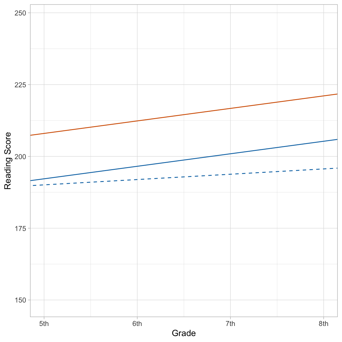
Since the model was based on grade level being centered at the initial measurement occasion, we need to use the centered grade in the x= argument of the ggplot() aesthetic mapping. Then we can re-label the x-scale to our original grade levels for easier interpretation for readers.
Interaction Between Grade and Special Education Status
Model D included grade-level and special education status as fixed-effects. This produces average growth profiles that have the same rate-of-growth for special education students and non-special education students. Substantively, the reason those students have different average reading scores is that they have different averages at the initial measurement occasion.
The model presumes that special education and non-special education students have, on average, the same growth rate over the duration of the study (5th through 8th grade).1 This is probably not a realistic assumption. We can allow different rates-of-growth by including an interaction between grade-level and special education status in addition to the main effects. The statistical model can be expressed as:
\[ \mathrm{Reading~Score}_{ij} = \big[\beta_0 + b_{0j}\big] + \big[\beta_1 + b_{1j}\big](\mathrm{Grade}_{ij}-5) + \beta_2(\mathrm{Special~Education}_j) + \beta_3(\mathrm{Grade}_{ij}-5)(\mathrm{Special~Education}_j) + \epsilon_{ij} \]
where,
- \(\mathrm{Reading~Score}_{ij}\) is the reading score for Student j at time point i;
- \(\beta_0\) is the fixed-effect of intercept;
- \(b_{0j}\) is the random-effect of intercept for Student j;
- \(\beta_1\) is the fixed-effect of grade-level;
- \(b_{1j}\) is the random-effect of grade-level for Student j;
- \(\beta_2\) is the fixed-effect of special education status;
- \(\beta_3\) is the interaction-effect (fixed-effect) between special education status grade-level; and
- \(\epsilon_{ij}\) is the error for Student j at time point i.
We fit the model using ML estimation, obtain both the fixed-effect estimates and estimated variance components, and add these results to our table of regression results.
# Fit model
lmer.e = lmer(reading_score ~ 1 + I(grade-5) + sped + I(grade-5):sped +
                (1 + I(grade-5) | student_id), data = mpls, REML = FALSE)

# Coefficient-level output
tidy(lmer.e, effects = "fixed")
# Obtain variance estimates
tidy(lmer.e, effects = "ran_pars")Code
htmlreg(
  l = list(lmer.a, lmer.b, lmer.c, lmer.d, lmer.e),
  stars = numeric(0),    #No p-value stars
  digits = 2,
  padding = 20, #Add space around columns (you may need to adjust this via trial-and-error)
  custom.model.names = c("Model A", "Model B", "Model C", "Model D", "Model E"),
  custom.coef.names = c("Intercept", "Grade", "Special Education Status", "Grade x Special Education Status"),
  reorder.coef = c(2:4, 1), #Put intercept at bottom of table
  include.loglik = FALSE, #Omit log-likelihood
  include.aic = FALSE,    #Omit AIC
  include.bic = FALSE,    #Omit BIC
  include.nobs = FALSE,   #Omit sample size
  include.groups = FALSE, #Omit group size
  include.deviance = TRUE,
  custom.gof.names = c("Deviance", "Level-2 Variance (Intercept)", "Level-1 Variance", "Level-2 Variance (Slope)", "Level-2 Covariance"), # Rename variance component rows
  custom.gof.rows = list(
    AICc = c(AICc(lmer.a), AICc(lmer.b), AICc(lmer.c), AICc(lmer.d), AICc(lmer.e))  # Add AICc values
  ),
  reorder.gof = c(3, 5, 6, 4, 2, 1),
  caption = NULL,
  caption.above = TRUE, #Move caption above table
  inner.rules = 1, #Include line rule before model-level output
  outer.rules = 1 , #Include line rules around table
  custom.note = "*Note.* The grade predictor was centered at the initial measurement occasion of 5th-grade. Special education status was dummy-coded using non-special education students as the reference group."
)| Model A | Model B | Model C | Model D | Model E | |
|---|---|---|---|---|---|
| Grade | 4.36 | 4.36 | 4.36 | 4.11 | |
| (0.52) | (0.70) | (0.70) | (0.74) | ||
| Special Education Status | -15.77 | -19.40 | |||
| (10.96) | (11.61) | ||||
| Grade x Special Education Status | 1.89 | ||||
| (2.01) | |||||
| Intercept | 212.64 | 206.09 | 206.09 | 208.24 | 208.74 |
| (3.96) | (4.04) | (4.23) | (4.26) | (4.29) | |
| Level-2 Variance (Intercept) | 329.66 | 337.57 | 381.44 | 338.62 | 337.07 |
| Level-2 Variance (Slope) | 7.38 | 7.38 | 6.96 | ||
| Level-2 Covariance | -19.12 | -15.60 | -14.79 | ||
| Level-1 Variance | 61.62 | 29.89 | 17.59 | 17.59 | 17.59 |
| Deviance | 680.78 | 633.02 | 622.52 | 620.61 | 619.74 |
| AICc | 687.07 | 641.50 | 635.56 | 636.01 | 637.56 |
| Note. The grade predictor was centered at the initial measurement occasion of 5th-grade. Special education status was dummy-coded using non-special education students as the reference group. | |||||
Taxonomy of models predicting longitudinal variation in students' reading scores.
The fitted equation for the average model is:
\[ \mathrm{Reading~Score}_{ij} = 209 + 4.11(\mathrm{Grade}_{ij}-5) - 19.4(\mathrm{Special~Education}_j) + 1.89(\mathrm{Grade}_{ij}-5)(\mathrm{Special~Education}_j) \]
The interaction effect is interpreted like any other interaction effect, either
- The effect of grade-level on reading scores varies by special education status. OR
- The effect of special education status on reading scores varies by grade-level.
To better understand this interaction, we can write out and then plot the average fitted equation for special education students and that for non-special education students.
\[ \begin{split} \mathbf{Non\mbox{-}SpEd:~}\mathrm{Reading~Score}_{ij} &= 209 + 4.11(\mathrm{Grade}_{ij}-5) - 19.4(0) + 1.89(\mathrm{Grade}_{ij}-5)(0) \\[1ex] &= 209 + 4.11(\mathrm{Grade}_{ij}-5) \\[4ex] \mathbf{SpEd:~}\mathrm{Reading~Score}_{ij} &= 209 + 4.11(\mathrm{Grade}_{ij}-5) - 19.4(1) + 1.89(\mathrm{Grade}_{ij}-5)(1) \\[1ex] &= 189.6 + 6.00(\mathrm{Grade}_{ij}-5) \end{split} \]
ggplot(data = mpls, aes(x = grade-5, y = reading_score)) +
  geom_point(alpha = 0) +  #Add individual profiles
  geom_abline(intercept = 209, slope = 4.11, color = "#D55E00") + #Non-Sped
  geom_abline(intercept = 189.6, slope = 6.00, color = "#0072B2") + #Sped
  theme_light() +
  scale_x_continuous(
    name = "Grade",
    breaks = c(0, 1, 2, 3),
    labels = c("5th", "6th", "7th", "8th")
    ) +
  ylab("Reading Score")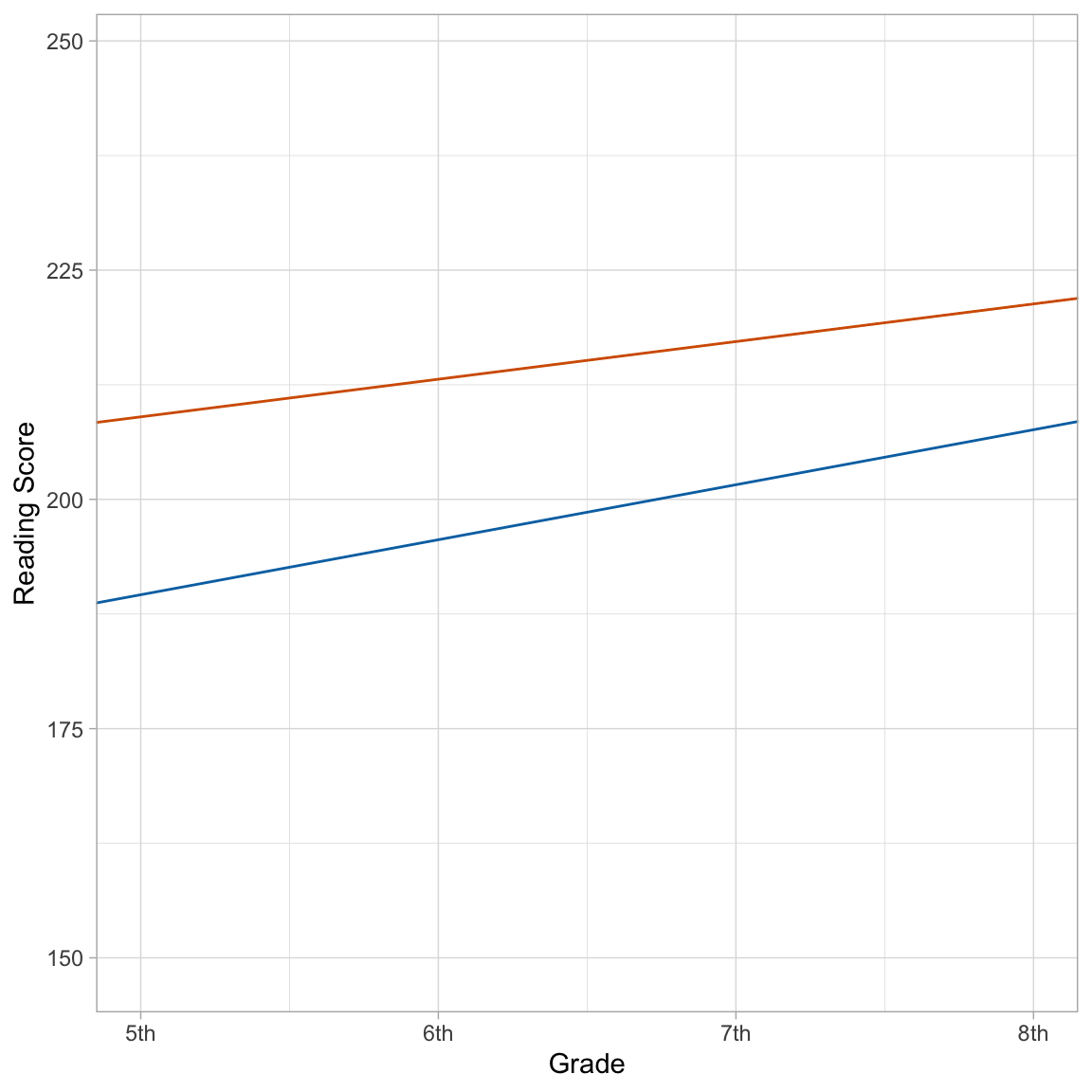
Non-special education students have a higher average reading score in the 5th grade than special education students. Moreover, they continue to have a higher average reading score than their special education peers throughout the duration of the study. However, the gap in reading scores gets smaller over time since the growth rate for special education students is higher than that for non-special education students.
Controlling for Attendance
We will fit one additional model that adds to Model E by controlling for attendance. The statistical model can be expressed as:
\[ \begin{split} \mathrm{Reading~Score}_{ij} = &\big[\beta_0 + b_{0j}\big] + \big[\beta_1 + b_{1j}\big](\mathrm{Grade}_{ij}-5) + \beta_2(\mathrm{Special~Education}_j) + \beta_3(\mathrm{Attendance}_j) + \\ &\beta_4(\mathrm{Grade}_{ij}-5)(\mathrm{Special~Education}_j) + \epsilon_{ij} \end{split} \]
where,
- \(\mathrm{Reading~Score}_{ij}\) is the reading score for Student j at time point i;
- \(\beta_0\) is the fixed-effect of intercept;
- \(b_{0j}\) is the random-effect of intercept for Student j;
- \(\beta_1\) is the fixed-effect of grade-level;
- \(\mathrm{Grade}_{ij}\) is the grade-level for Student j at time point i;
- \(b_{1j}\) is the random-effect of grade-level for Student j;
- \(\beta_2\) is the fixed-effect of special education status;
- \(\mathrm{Special~Education}_{j}\) is the dummy-coded special education status for Student j
- \(\beta_3\) is the fixed-effect of attendance;
- \(\mathrm{Attendance}_{j}\) is the attendance for Student j
- \(\beta_4\) is the interaction-effect (fixed-effect) between special education status grade-level; and
- \(\epsilon_{ij}\) is the error for Student j at time point i.
We fit the model using ML estimation, obtain both the fixed-effect estimates and estimated variance components, and add these results to our table of regression results. To facilitate better interpretation of the intercept, we will mean center the attendance variable.
# Fit model
lmer.f = lmer(reading_score ~ 1 + I(grade-5) + sped + I(attendance - 0.9564) + I(grade-5):sped +
                (1 + I(grade-5) | student_id), data = mpls, REML = FALSE)

# Coefficient-level output
tidy(lmer.f, effects = "fixed")
# Obtain variance estimates
tidy(lmer.f, effects = "ran_pars")Code
htmlreg(
  l = list(lmer.a, lmer.b, lmer.c, lmer.d, lmer.e, lmer.f),
  stars = numeric(0),    #No p-value stars
  digits = 2,
  padding = 20, #Add space around columns (you may need to adjust this via trial-and-error)
  custom.model.names = c("Model A", "Model B", "Model C", "Model D", "Model E", "Model F"),
  custom.coef.names = c("Intercept", "Grade", "Special Education Status", "Attendance",
                        "Grade x Special Education Status"),
  reorder.coef = c(2:5, 1), #Put intercept at bottom of table
  include.loglik = FALSE, #Omit log-likelihood
  include.aic = FALSE,    #Omit AIC
  include.bic = FALSE,    #Omit BIC
  include.nobs = FALSE,   #Omit sample size
  include.groups = FALSE, #Omit group size
  include.deviance = TRUE,
  custom.gof.names = c("Deviance", "Level-2 Variance (Intercept)", "Level-1 Variance", "Level-2 Variance (Slope)", "Level-2 Covariance"), # Rename variance component rows
  custom.gof.rows = list(
    AICc = c(AICc(lmer.a), AICc(lmer.b), AICc(lmer.c), AICc(lmer.d), AICc(lmer.e), AICc(lmer.f))  # Add AICc values
  ),
  reorder.gof = c(3, 5, 6, 4, 2, 1),
  caption = NULL,
  caption.above = TRUE, #Move caption above table
  inner.rules = 1, #Include line rule before model-level output
  outer.rules = 1 , #Include line rules around table
  custom.note = "*Note.* The grade predictor was centered at the initial measurement occasion of 5th-grade. Special education status was dummy-coded using non-special education students as the reference group. The attendance variable was mean centered."
)| Model A | Model B | Model C | Model D | Model E | Model F | |
|---|---|---|---|---|---|---|
| Grade | 4.36 | 4.36 | 4.36 | 4.11 | 4.11 | |
| (0.52) | (0.70) | (0.70) | (0.74) | (0.74) | ||
| Special Education Status | -15.77 | -19.40 | -22.01 | |||
| (10.96) | (11.61) | (11.38) | ||||
| Attendance | 1.89 | 1.89 | ||||
| (2.01) | (2.01) | |||||
| Grade x Special Education Status | 218.39 | |||||
| (89.83) | ||||||
| Intercept | 212.64 | 206.09 | 206.09 | 208.24 | 208.74 | 209.10 |
| (3.96) | (4.04) | (4.23) | (4.26) | (4.29) | (4.18) | |
| Level-2 Variance (Intercept) | 329.66 | 337.57 | 381.44 | 338.62 | 337.07 | 320.00 |
| Level-2 Variance (Slope) | 7.38 | 7.38 | 6.96 | 6.96 | ||
| Level-2 Covariance | -19.12 | -15.60 | -14.79 | -23.85 | ||
| Level-1 Variance | 61.62 | 29.89 | 17.59 | 17.59 | 17.59 | 17.59 |
| Deviance | 680.78 | 633.02 | 622.52 | 620.61 | 619.74 | 615.05 |
| AICc | 687.07 | 641.50 | 635.56 | 636.01 | 637.56 | 635.36 |
| Note. The grade predictor was centered at the initial measurement occasion of 5th-grade. Special education status was dummy-coded using non-special education students as the reference group. The attendance variable was mean centered. | ||||||
Taxonomy of models predicting longitudinal variation in students' reading scores.
The fitted equation for the average model is:
\[ \begin{split} \mathrm{Reading~Score}_{ij} = &209 + 4.11(\mathrm{Grade}_{ij}-5) - 22(\mathrm{Special~Education}_j) + 218(\mathrm{Attendance}_j) +\\ &1.89(\mathrm{Grade}_{ij}-5)(\mathrm{Special~Education}_j) \end{split} \]
Interpreting the interaction effect:
- The effect of grade-level on reading scores varies by special education status after controlling for differences in attendance. OR
- The effect of special education status on reading scores varies by grade-level after controlling for differences in attendance.
To better understand this interaction, we can write out and then plot the average fitted equation for special education students and that for non-special education students. We will control for attendance by setting it to its mean value. Note that since we mean centered attendance, this will drop the attendance term from the fitted equation.
\[ \begin{split} \mathbf{Non\mbox{-}SpEd:~}\mathrm{Reading~Score}_{ij} &= 209 + 4.11(\mathrm{Grade}_{ij}-5) - 22(0) + 218(0.9564 - 0.9564) + 1.89(\mathrm{Grade}_{ij}-5)(0) \\[1ex] &= 209 + 4.11(\mathrm{Grade}_{ij}-5) \\[4ex] \mathbf{SpEd:~}\mathrm{Reading~Score}_{ij} &= 209 + 4.11(\mathrm{Grade}_{ij}-5) - 22(1) + 218(0.9564 - 0.9564) + 1.89(\mathrm{Grade}_{ij}-5)(1) \\[1ex] &= 187 + 6.00(\mathrm{Grade}_{ij}-5) \end{split} \]
This results in essentially the same plot as Model E (the special education students profile will have a slightly lower reading score in the 5th grade). The difference is now the profiles represent the growth in reading scores for special education and non special education students who have an average attendance. Student specific fitted equations would have to be computed using the student’s special education status and the student’s actual attendance, as well as their random-effects.
Adopting a Model
We can use information criteria to select from out six candidate models since each model has the same outcome and has used the same data.
# Model evidence
aictab(
  cand.set = list(lmer.a, lmer.b, lmer.c, lmer.d, lmer.e, lmer.f),
  modnames = c("Model A", "Model B", "Model C", "Model D", "Model E", "Model F")
)
Given the data and candidate set of models, Model F has the most empirical evidence. However, there also seems to be a fair amount of evidence for Models C, D, and E. All of these models included random-effects of both intercept and slope.
Rocking a Prettier Table of Regression Results
While the table of regression results produced by htmlreg() is fine, there are several small tweaks that we might want to make, including:
- Rows indicating the fixed-effects, variance components, and model-level summaries
- Some horizontal guide lines to separate these sections
When you run the htmlreg() syntax, it produces the HTML syntax that is used to create the table. Embedding this in a code chunk with the option results='asis' will actually render the HTML syntax and produce the table in the resulting HTML file.
One way of customizing the output is to modify the HTML syntax. To do this we run the htmlreg() in the Console and copy and paste it into our RMD file. (Paste this syntax outside of a code chunk!)
# View HTML code
htmlreg(
  l = list(lmer.a, lmer.b, lmer.c, lmer.d, lmer.e, lmer.f),
  stars = numeric(0),    #No p-value stars
  digits = 2,
  padding = 20, #Add space around columns (you may need to adjust this via trial-and-error)
  custom.model.names = c("Model A", "Model B", "Model C", "Model D", "Model E", "Model F"),
  custom.coef.names = c("Intercept", "Grade", "Special Education Status", "Attendance",
                        "Grade x Special Education Status"),
  reorder.coef = c(2:5, 1), #Put intercept at bottom of table
  include.loglik = FALSE, #Omit log-likelihood
  include.aic = FALSE,    #Omit AIC
  include.bic = FALSE,    #Omit BIC
  include.nobs = FALSE,   #Omit sample size
  include.groups = FALSE, #Omit group size
  include.deviance = TRUE,
  custom.gof.names = c("Deviance", "Level-2 (Intercept)", "Level-1", "Level-2 (Slope)", "Level-2 Covariance"), # Rename variance component rows
  custom.gof.rows = list(
    AICc = c(AICc(lmer.a), AICc(lmer.b), AICc(lmer.c), AICc(lmer.d), AICc(lmer.e), AICc(lmer.f))  # Add AICc values
  ),
  reorder.gof = c(3, 5, 6, 4, 2, 1),
  caption = "Taxonomy of models predicting longitudinal variation in students' reading scores.",
  caption.above = TRUE, #Move caption above table
  inner.rules = 1, #Include line rule before model-level output
  outer.rules = 1 , #Include line rules around table
  custom.note = "*Note.* The grade predictor was centered at the initial measurement occasion of 5th-grade. Special education status was dummy-coded using non-special education students as the reference group. The attendance variable was mean centered."
)
<table class="texreg" style="margin: 10px auto;border-collapse: collapse;border-spacing: 0px;color: #000000;border-top: 1px solid #000000;">
<caption>Taxonomy of models predicting longitudinal variation in students' reading scores.</caption>
<thead>
<tr>
<th style="padding-left: 20px;padding-right: 20px;"> </th>
<th style="padding-left: 20px;padding-right: 20px;">Model A</th>
<th style="padding-left: 20px;padding-right: 20px;">Model B</th>
<th style="padding-left: 20px;padding-right: 20px;">Model C</th>
<th style="padding-left: 20px;padding-right: 20px;">Model D</th>
<th style="padding-left: 20px;padding-right: 20px;">Model E</th>
<th style="padding-left: 20px;padding-right: 20px;">Model F</th>
</tr>
</thead>
<tbody>
<tr style="border-top: 1px solid #000000;">
<td style="padding-left: 20px;padding-right: 20px;">Grade</td>
<td style="padding-left: 20px;padding-right: 20px;"> </td>
<td style="padding-left: 20px;padding-right: 20px;">4.36</td>
<td style="padding-left: 20px;padding-right: 20px;">4.36</td>
<td style="padding-left: 20px;padding-right: 20px;">4.36</td>
<td style="padding-left: 20px;padding-right: 20px;">4.11</td>
<td style="padding-left: 20px;padding-right: 20px;">4.11</td>
</tr>
<tr>
<td style="padding-left: 20px;padding-right: 20px;"> </td>
<td style="padding-left: 20px;padding-right: 20px;"> </td>
<td style="padding-left: 20px;padding-right: 20px;">(0.52)</td>
<td style="padding-left: 20px;padding-right: 20px;">(0.70)</td>
<td style="padding-left: 20px;padding-right: 20px;">(0.70)</td>
<td style="padding-left: 20px;padding-right: 20px;">(0.74)</td>
<td style="padding-left: 20px;padding-right: 20px;">(0.74)</td>
</tr>
<tr>
<td style="padding-left: 20px;padding-right: 20px;">Special Education Status</td>
<td style="padding-left: 20px;padding-right: 20px;"> </td>
<td style="padding-left: 20px;padding-right: 20px;"> </td>
<td style="padding-left: 20px;padding-right: 20px;"> </td>
<td style="padding-left: 20px;padding-right: 20px;">-15.77</td>
<td style="padding-left: 20px;padding-right: 20px;">-19.40</td>
<td style="padding-left: 20px;padding-right: 20px;">-22.01</td>
</tr>
<tr>
<td style="padding-left: 20px;padding-right: 20px;"> </td>
<td style="padding-left: 20px;padding-right: 20px;"> </td>
<td style="padding-left: 20px;padding-right: 20px;"> </td>
<td style="padding-left: 20px;padding-right: 20px;"> </td>
<td style="padding-left: 20px;padding-right: 20px;">(10.96)</td>
<td style="padding-left: 20px;padding-right: 20px;">(11.61)</td>
<td style="padding-left: 20px;padding-right: 20px;">(11.38)</td>
</tr>
<tr>
<td style="padding-left: 20px;padding-right: 20px;">Attendance</td>
<td style="padding-left: 20px;padding-right: 20px;"> </td>
<td style="padding-left: 20px;padding-right: 20px;"> </td>
<td style="padding-left: 20px;padding-right: 20px;"> </td>
<td style="padding-left: 20px;padding-right: 20px;"> </td>
<td style="padding-left: 20px;padding-right: 20px;">1.89</td>
<td style="padding-left: 20px;padding-right: 20px;">1.89</td>
</tr>
<tr>
<td style="padding-left: 20px;padding-right: 20px;"> </td>
<td style="padding-left: 20px;padding-right: 20px;"> </td>
<td style="padding-left: 20px;padding-right: 20px;"> </td>
<td style="padding-left: 20px;padding-right: 20px;"> </td>
<td style="padding-left: 20px;padding-right: 20px;"> </td>
<td style="padding-left: 20px;padding-right: 20px;">(2.01)</td>
<td style="padding-left: 20px;padding-right: 20px;">(2.01)</td>
</tr>
<tr>
<td style="padding-left: 20px;padding-right: 20px;">Grade x Special Education Status</td>
<td style="padding-left: 20px;padding-right: 20px;"> </td>
<td style="padding-left: 20px;padding-right: 20px;"> </td>
<td style="padding-left: 20px;padding-right: 20px;"> </td>
<td style="padding-left: 20px;padding-right: 20px;"> </td>
<td style="padding-left: 20px;padding-right: 20px;"> </td>
<td style="padding-left: 20px;padding-right: 20px;">218.39</td>
</tr>
<tr>
<td style="padding-left: 20px;padding-right: 20px;"> </td>
<td style="padding-left: 20px;padding-right: 20px;"> </td>
<td style="padding-left: 20px;padding-right: 20px;"> </td>
<td style="padding-left: 20px;padding-right: 20px;"> </td>
<td style="padding-left: 20px;padding-right: 20px;"> </td>
<td style="padding-left: 20px;padding-right: 20px;"> </td>
<td style="padding-left: 20px;padding-right: 20px;">(89.83)</td>
</tr>
<tr>
<td style="padding-left: 20px;padding-right: 20px;">Intercept</td>
<td style="padding-left: 20px;padding-right: 20px;">212.64</td>
<td style="padding-left: 20px;padding-right: 20px;">206.09</td>
<td style="padding-left: 20px;padding-right: 20px;">206.09</td>
<td style="padding-left: 20px;padding-right: 20px;">208.24</td>
<td style="padding-left: 20px;padding-right: 20px;">208.74</td>
<td style="padding-left: 20px;padding-right: 20px;">209.10</td>
</tr>
<tr>
<td style="padding-left: 20px;padding-right: 20px;"> </td>
<td style="padding-left: 20px;padding-right: 20px;">(3.96)</td>
<td style="padding-left: 20px;padding-right: 20px;">(4.04)</td>
<td style="padding-left: 20px;padding-right: 20px;">(4.23)</td>
<td style="padding-left: 20px;padding-right: 20px;">(4.26)</td>
<td style="padding-left: 20px;padding-right: 20px;">(4.29)</td>
<td style="padding-left: 20px;padding-right: 20px;">(4.18)</td>
</tr>
<tr style="border-top: 1px solid #000000;">
<td style="padding-left: 20px;padding-right: 20px;">Level-2 (Intercept)</td>
<td style="padding-left: 20px;padding-right: 20px;">329.66</td>
<td style="padding-left: 20px;padding-right: 20px;">337.57</td>
<td style="padding-left: 20px;padding-right: 20px;">381.44</td>
<td style="padding-left: 20px;padding-right: 20px;">338.62</td>
<td style="padding-left: 20px;padding-right: 20px;">337.07</td>
<td style="padding-left: 20px;padding-right: 20px;">320.00</td>
</tr>
<tr>
<td style="padding-left: 20px;padding-right: 20px;">Level-2 (Slope)</td>
<td style="padding-left: 20px;padding-right: 20px;"> </td>
<td style="padding-left: 20px;padding-right: 20px;"> </td>
<td style="padding-left: 20px;padding-right: 20px;">7.38</td>
<td style="padding-left: 20px;padding-right: 20px;">7.38</td>
<td style="padding-left: 20px;padding-right: 20px;">6.96</td>
<td style="padding-left: 20px;padding-right: 20px;">6.96</td>
</tr>
<tr>
<td style="padding-left: 20px;padding-right: 20px;">Level-2 Covariance</td>
<td style="padding-left: 20px;padding-right: 20px;"> </td>
<td style="padding-left: 20px;padding-right: 20px;"> </td>
<td style="padding-left: 20px;padding-right: 20px;">-19.12</td>
<td style="padding-left: 20px;padding-right: 20px;">-15.60</td>
<td style="padding-left: 20px;padding-right: 20px;">-14.79</td>
<td style="padding-left: 20px;padding-right: 20px;">-23.85</td>
</tr>
<tr>
<td style="padding-left: 20px;padding-right: 20px;">Level-1</td>
<td style="padding-left: 20px;padding-right: 20px;">61.62</td>
<td style="padding-left: 20px;padding-right: 20px;">29.89</td>
<td style="padding-left: 20px;padding-right: 20px;">17.59</td>
<td style="padding-left: 20px;padding-right: 20px;">17.59</td>
<td style="padding-left: 20px;padding-right: 20px;">17.59</td>
<td style="padding-left: 20px;padding-right: 20px;">17.59</td>
</tr>
<tr>
<td style="padding-left: 20px;padding-right: 20px;">Deviance</td>
<td style="padding-left: 20px;padding-right: 20px;">680.78</td>
<td style="padding-left: 20px;padding-right: 20px;">633.02</td>
<td style="padding-left: 20px;padding-right: 20px;">622.52</td>
<td style="padding-left: 20px;padding-right: 20px;">620.61</td>
<td style="padding-left: 20px;padding-right: 20px;">619.74</td>
<td style="padding-left: 20px;padding-right: 20px;">615.05</td>
</tr>
<tr style="border-bottom: 1px solid #000000;">
<td style="padding-left: 20px;padding-right: 20px;">AICc</td>
<td style="padding-left: 20px;padding-right: 20px;">687.07</td>
<td style="padding-left: 20px;padding-right: 20px;">641.50</td>
<td style="padding-left: 20px;padding-right: 20px;">635.56</td>
<td style="padding-left: 20px;padding-right: 20px;">636.01</td>
<td style="padding-left: 20px;padding-right: 20px;">637.56</td>
<td style="padding-left: 20px;padding-right: 20px;">635.36</td>
</tr>
</tbody>
<tfoot>
<tr>
<td style="font-size: 0.8em;" colspan="7">*Note.* The grade predictor was centered at the initial measurement occasion of 5th-grade. Special education status was dummy-coded using non-special education students as the reference group. The attendance variable was mean centered.</td>
</tr>
</tfoot>
</table>If you are going to create the table by modifying the HTML, you should set the caption= argument in htmlreg() to the caption you want.
HTML code consists of tags that define certain features. There is typically an opening tag <tag> and a closing tag </tag>. The tags in the syntax produced by htmlreg() are all related to producing different features of a table:
<table>and</table>define a table<caption>and</caption>define a the table caption<thead>and</thead>define the table header<tbody>and</tbody>define the table body<tfoot>and</tfoot>define the table footer<tr>and</tr>define a table row<td>and</td>define a cell (table data) in a row (Note that in the header we use<th>and</th>. This makes the cell content bold by default.)
Within these tags their are certain arguments (called attributes in the HTML nomenclature). The most common is the style= attribute. This conisists of CSS syntax that styles the contents of the tag. For example, the syntax:
<td style="padding-left: 20px;padding-right: 20px;">Grade</td>produces a cell in the table that includes the content ‘Grade’. The CSS syntax in style= includes both left- and right-side padding to include space around the cell content.
We will manually include additional HTML and CSS syntax to the existing table syntax to customize our output. For example to add a row that includes the text Fixed-effects and also includes a top border (horizontal guide line), we use:
<tr style="border-top: 1px solid #000000;">
  <td style="text-align: center; padding-top:5px; padding-bottom:10px;" colspan="7">Fixed-effects
</tr>
This adds a row with top border that is 1 pixel thick, solid, and black. The text in th cell will be centered and have some padding space above and below the text (this allows the content of the row to breathe). The colspan="7" attribute spans the cell content across all seven columns of the table.
I have added this to include a row to indicate ‘Fixed-effects’. ‘Random-effects (Variance components)’, and ‘Model-level summaries’. (You can view the syntax used in the RMD file. I have included comments to indicate where these rows are added.)
Code
<!-- MODIFIED TABLE -->
<table class="texreg" style="margin: 10px auto;border-collapse: collapse;border-spacing: 0px;color: #000000;border-top: 1px solid #000000;">
<caption>Taxonomy of models predicting longitudinal variation in students' reading scores.</caption>
<thead>
<tr>
<th style="padding-left: 20px;padding-right: 20px;"> </th>
<th style="padding-left: 20px;padding-right: 20px;">Model A</th>
<th style="padding-left: 20px;padding-right: 20px;">Model B</th>
<th style="padding-left: 20px;padding-right: 20px;">Model C</th>
<th style="padding-left: 20px;padding-right: 20px;">Model D</th>
<th style="padding-left: 20px;padding-right: 20px;">Model E</th>
<th style="padding-left: 20px;padding-right: 20px;">Model F</th>
</tr>
</thead>
<tbody>
<!-- Add row indicating fixed-effects -->
<tr style="border-top: 1px solid #000000;">
<td style="text-align: center; padding-top:5px; padding-bottom:10px;" colspan="7">Fixed-effects
</tr>
<!-- In the next row, we remove the border that was there so we don't get a double border -->
<tr>
<td style="padding-left: 20px;padding-right: 20px;">Grade</td>
<td style="padding-left: 20px;padding-right: 20px;"> </td>
<td style="padding-left: 20px;padding-right: 20px;">4.36</td>
<td style="padding-left: 20px;padding-right: 20px;">4.36</td>
<td style="padding-left: 20px;padding-right: 20px;">4.36</td>
<td style="padding-left: 20px;padding-right: 20px;">4.11</td>
<td style="padding-left: 20px;padding-right: 20px;">4.11</td>
</tr>
<tr>
<td style="padding-left: 20px;padding-right: 20px;"> </td>
<td style="padding-left: 20px;padding-right: 20px;"> </td>
<td style="padding-left: 20px;padding-right: 20px;">(0.52)</td>
<td style="padding-left: 20px;padding-right: 20px;">(0.70)</td>
<td style="padding-left: 20px;padding-right: 20px;">(0.70)</td>
<td style="padding-left: 20px;padding-right: 20px;">(0.74)</td>
<td style="padding-left: 20px;padding-right: 20px;">(0.74)</td>
</tr>
<tr>
<td style="padding-left: 20px;padding-right: 20px;">Special Education Status</td>
<td style="padding-left: 20px;padding-right: 20px;"> </td>
<td style="padding-left: 20px;padding-right: 20px;"> </td>
<td style="padding-left: 20px;padding-right: 20px;"> </td>
<td style="padding-left: 20px;padding-right: 20px;">-15.77</td>
<td style="padding-left: 20px;padding-right: 20px;">-19.40</td>
<td style="padding-left: 20px;padding-right: 20px;">-22.01</td>
</tr>
<tr>
<td style="padding-left: 20px;padding-right: 20px;"> </td>
<td style="padding-left: 20px;padding-right: 20px;"> </td>
<td style="padding-left: 20px;padding-right: 20px;"> </td>
<td style="padding-left: 20px;padding-right: 20px;"> </td>
<td style="padding-left: 20px;padding-right: 20px;">(10.96)</td>
<td style="padding-left: 20px;padding-right: 20px;">(11.61)</td>
<td style="padding-left: 20px;padding-right: 20px;">(11.38)</td>
</tr>
<tr>
<td style="padding-left: 20px;padding-right: 20px;">Attendance</td>
<td style="padding-left: 20px;padding-right: 20px;"> </td>
<td style="padding-left: 20px;padding-right: 20px;"> </td>
<td style="padding-left: 20px;padding-right: 20px;"> </td>
<td style="padding-left: 20px;padding-right: 20px;"> </td>
<td style="padding-left: 20px;padding-right: 20px;">1.89</td>
<td style="padding-left: 20px;padding-right: 20px;">1.89</td>
</tr>
<tr>
<td style="padding-left: 20px;padding-right: 20px;"> </td>
<td style="padding-left: 20px;padding-right: 20px;"> </td>
<td style="padding-left: 20px;padding-right: 20px;"> </td>
<td style="padding-left: 20px;padding-right: 20px;"> </td>
<td style="padding-left: 20px;padding-right: 20px;"> </td>
<td style="padding-left: 20px;padding-right: 20px;">(2.01)</td>
<td style="padding-left: 20px;padding-right: 20px;">(2.01)</td>
</tr>
<tr>
<td style="padding-left: 20px;padding-right: 20px;">Grade x Special Education Status</td>
<td style="padding-left: 20px;padding-right: 20px;"> </td>
<td style="padding-left: 20px;padding-right: 20px;"> </td>
<td style="padding-left: 20px;padding-right: 20px;"> </td>
<td style="padding-left: 20px;padding-right: 20px;"> </td>
<td style="padding-left: 20px;padding-right: 20px;"> </td>
<td style="padding-left: 20px;padding-right: 20px;">218.39</td>
</tr>
<tr>
<td style="padding-left: 20px;padding-right: 20px;"> </td>
<td style="padding-left: 20px;padding-right: 20px;"> </td>
<td style="padding-left: 20px;padding-right: 20px;"> </td>
<td style="padding-left: 20px;padding-right: 20px;"> </td>
<td style="padding-left: 20px;padding-right: 20px;"> </td>
<td style="padding-left: 20px;padding-right: 20px;"> </td>
<td style="padding-left: 20px;padding-right: 20px;">(89.83)</td>
</tr>
<tr>
<td style="padding-left: 20px;padding-right: 20px;">Intercept</td>
<td style="padding-left: 20px;padding-right: 20px;">212.64</td>
<td style="padding-left: 20px;padding-right: 20px;">206.09</td>
<td style="padding-left: 20px;padding-right: 20px;">206.09</td>
<td style="padding-left: 20px;padding-right: 20px;">208.24</td>
<td style="padding-left: 20px;padding-right: 20px;">208.74</td>
<td style="padding-left: 20px;padding-right: 20px;">209.10</td>
</tr>
<tr>
<td style="padding-left: 20px;padding-right: 20px;"> </td>
<td style="padding-left: 20px;padding-right: 20px;">(3.96)</td>
<td style="padding-left: 20px;padding-right: 20px;">(4.04)</td>
<td style="padding-left: 20px;padding-right: 20px;">(4.23)</td>
<td style="padding-left: 20px;padding-right: 20px;">(4.26)</td>
<td style="padding-left: 20px;padding-right: 20px;">(4.29)</td>
<td style="padding-left: 20px;padding-right: 20px;">(4.18)</td>
</tr>
<!-- Add row indicating random-effects -->
<tr style="border-top: 1px solid #000000;">
<td style="text-align: center; padding-top:5px; padding-bottom:10px;" colspan="7">Random-effects (Variance Components)
</tr>
<!-- In the next row, we remove the border that was there so we don't get a double border -->
<tr>
<td style="padding-left: 20px;padding-right: 20px;">Level-2 (Intercept)</td>
<td style="padding-left: 20px;padding-right: 20px;">329.66</td>
<td style="padding-left: 20px;padding-right: 20px;">337.57</td>
<td style="padding-left: 20px;padding-right: 20px;">381.44</td>
<td style="padding-left: 20px;padding-right: 20px;">338.62</td>
<td style="padding-left: 20px;padding-right: 20px;">337.07</td>
<td style="padding-left: 20px;padding-right: 20px;">320.00</td>
</tr>
<tr>
<td style="padding-left: 20px;padding-right: 20px;">Level-2 (Slope)</td>
<td style="padding-left: 20px;padding-right: 20px;"> </td>
<td style="padding-left: 20px;padding-right: 20px;"> </td>
<td style="padding-left: 20px;padding-right: 20px;">7.38</td>
<td style="padding-left: 20px;padding-right: 20px;">7.38</td>
<td style="padding-left: 20px;padding-right: 20px;">6.96</td>
<td style="padding-left: 20px;padding-right: 20px;">6.96</td>
</tr>
<tr>
<td style="padding-left: 20px;padding-right: 20px;">Level-2 Covariance</td>
<td style="padding-left: 20px;padding-right: 20px;"> </td>
<td style="padding-left: 20px;padding-right: 20px;"> </td>
<td style="padding-left: 20px;padding-right: 20px;">-19.12</td>
<td style="padding-left: 20px;padding-right: 20px;">-15.60</td>
<td style="padding-left: 20px;padding-right: 20px;">-14.79</td>
<td style="padding-left: 20px;padding-right: 20px;">-23.85</td>
</tr>
<tr>
<td style="padding-left: 20px;padding-right: 20px;">Level-1</td>
<td style="padding-left: 20px;padding-right: 20px;">61.62</td>
<td style="padding-left: 20px;padding-right: 20px;">29.89</td>
<td style="padding-left: 20px;padding-right: 20px;">17.59</td>
<td style="padding-left: 20px;padding-right: 20px;">17.59</td>
<td style="padding-left: 20px;padding-right: 20px;">17.59</td>
<td style="padding-left: 20px;padding-right: 20px;">17.59</td>
</tr>
<!-- Add row indicating model-level summaries-->
<tr style="border-top: 1px solid #000000;">
<td style="text-align: center; padding-top:5px; padding-bottom:10px;" colspan="7">Model-level summaries
</tr>
<tr>
<td style="padding-left: 20px;padding-right: 20px;">Deviance</td>
<td style="padding-left: 20px;padding-right: 20px;">680.78</td>
<td style="padding-left: 20px;padding-right: 20px;">633.02</td>
<td style="padding-left: 20px;padding-right: 20px;">622.52</td>
<td style="padding-left: 20px;padding-right: 20px;">620.61</td>
<td style="padding-left: 20px;padding-right: 20px;">619.74</td>
<td style="padding-left: 20px;padding-right: 20px;">615.05</td>
</tr>
<tr style="border-bottom: 1px solid #000000;">
<td style="padding-left: 20px;padding-right: 20px;">AICc</td>
<td style="padding-left: 20px;padding-right: 20px;">687.07</td>
<td style="padding-left: 20px;padding-right: 20px;">641.50</td>
<td style="padding-left: 20px;padding-right: 20px;">635.56</td>
<td style="padding-left: 20px;padding-right: 20px;">636.01</td>
<td style="padding-left: 20px;padding-right: 20px;">637.56</td>
<td style="padding-left: 20px;padding-right: 20px;">635.36</td>
</tr>
</tbody>
<tfoot>
<tr>
<td style="font-size: 0.8em;" colspan="7"><i>Note.</i> The grade predictor was centered at the initial measurement occasion of 5th-grade. Special education status was dummy-coded using non-special education students as the reference group. The attendance variable was mean centered.</td>
</tr>
</tfoot>
</table>| Model A | Model B | Model C | Model D | Model E | Model F | |
|---|---|---|---|---|---|---|
| Fixed-effects | ||||||
| Grade | 4.36 | 4.36 | 4.36 | 4.11 | 4.11 | |
| (0.52) | (0.70) | (0.70) | (0.74) | (0.74) | ||
| Special Education Status | -15.77 | -19.40 | -22.01 | |||
| (10.96) | (11.61) | (11.38) | ||||
| Attendance | 1.89 | 1.89 | ||||
| (2.01) | (2.01) | |||||
| Grade x Special Education Status | 218.39 | |||||
| (89.83) | ||||||
| Intercept | 212.64 | 206.09 | 206.09 | 208.24 | 208.74 | 209.10 |
| (3.96) | (4.04) | (4.23) | (4.26) | (4.29) | (4.18) | |
| Random-effects (Variance Components) | ||||||
| Level-2 (Intercept) | 329.66 | 337.57 | 381.44 | 338.62 | 337.07 | 320.00 |
| Level-2 (Slope) | 7.38 | 7.38 | 6.96 | 6.96 | ||
| Level-2 Covariance | -19.12 | -15.60 | -14.79 | -23.85 | ||
| Level-1 | 61.62 | 29.89 | 17.59 | 17.59 | 17.59 | 17.59 |
| Model-level summaries | ||||||
| Deviance | 680.78 | 633.02 | 622.52 | 620.61 | 619.74 | 615.05 |
| AICc | 687.07 | 641.50 | 635.56 | 636.01 | 637.56 | 635.36 |
| Note. The grade predictor was centered at the initial measurement occasion of 5th-grade. Special education status was dummy-coded using non-special education students as the reference group. The attendance variable was mean centered. | ||||||
Footnotes
Note that the random effects we included in Model D allow individual students to have different growth rates from the average growth rate.↩︎