Unit 6: Information Criteria for Model Selection
In this set of notes, you will learn about using information criteria to select a model from a set of candidate models.
Preparation
Before class you will need read the following:
- Elliott, L. P., & Brook, B. W. (2007). Revisiting Chamberlin: Multiple working hypotheses for the 21st century. BioScience, 57(7), 608–614.
6.1 Dataset and Research Question
In this set of notes, we will use the data in the ed-schools-2018.csv file (see the data codebook here). These data include institutional-level attributes for several graduate education schools/programs rated by U.S. News and World Report in 2018.
# Load libraries
library(broom)
library(corrr)
library(dplyr)
library(ggplot2)
library(readr)
library(sm)
library(tidyr)

# Read in data
ed = read_csv(file = "~/Documents/github/epsy-8252/data/ed-schools-2018.csv")
head(ed)
# A tibble: 6 x 13
rank school score peer expert_score gre_verbal gre_quant doc_accept
<dbl> <chr> <dbl> <dbl> <dbl> <dbl> <dbl> <dbl>
1 1 Harva… 100 4.4 4.6 163 159 4.5
2 2 Stanf… 99 4.6 4.8 162 160 6.1
3 3 Unive… 96 4.2 4.3 156 152 29.1
4 3 Unive… 96 4.1 4.5 163 157 5
5 3 Unive… 96 4.3 4.5 155 153 26.1
6 6 Johns… 95 4.1 4.1 164 162 27.4
# … with 5 more variables: phd_student_faculty_ratio <dbl>,
# phd_granted_per_faculty <dbl>, funded_research <dbl>,
# funded_research_per_faculty <dbl>, enroll <dbl>Using these data, we will examine the factors our academic peers use to rate graduate programs. To gather the peer assessment data, U.S. News asked deans, program directors and senior faculty to judge the academic quality of programs in their field on a scale of 1 (marginal) to 5 (outstanding). Based on the substantive literature we have three scientific working hypotheses about how programs are rated:
- H1: Student-related factors drive the perceived academic quality of graduate programs in education.
- H2: Faculty-related factors drive the perceived academic quality of graduate programs in education.
- H3: Institution-related factors drive the perceived academic quality of graduate programs in education.
We need to translate these working hypotheses into statistical models that we can then fit to a set of data. The models are only proxies for the working hypotheses. However, that being said, the validity of using the models as proxies is dependent on whether we have measured well, whether the translation makes substantive sense given the literature base, etc. Here is how we are measuring the different attributes:
- The student-related factors we will use are GRE scores.
- The faculty-related factors we will use are funded research (per faculty member) and the number of Ph.D. graduates (per faculty member).
- The institution-related factors we will use are the acceptance rate of Ph.D. students, the Ph.D. student-to-faculty ratio, and the size of the program.
6.2 Model-Building
Before we begin the exploratory analysis associated with model-building, it is worth noting that there are missing data in the dataset.
summary(ed) rank school score peer
Min. : 1.0 Length:129 Min. : 38.0 Min. :2.50
1st Qu.: 32.0 Class :character 1st Qu.: 42.0 1st Qu.:2.90
Median : 62.0 Mode :character Median : 51.0 Median :3.20
Mean : 63.2 Mean : 55.3 Mean :3.29
3rd Qu.: 93.0 3rd Qu.: 63.0 3rd Qu.:3.60
expert_score gre_verbal gre_quant doc_accept
Min. :2.40 Min. :148 Min. :142 Min. : 4.5
1st Qu.:3.30 1st Qu.:152 1st Qu.:148 1st Qu.: 25.8
Median :3.60 Median :154 Median :150 Median : 39.8
Mean :3.64 Mean :155 Mean :151 Mean : 41.4
3rd Qu.:4.00 3rd Qu.:156 3rd Qu.:153 3rd Qu.: 54.1
phd_student_faculty_ratio phd_granted_per_faculty funded_research
Min. : 0.00 Min. :0.000 Min. : 0.10
1st Qu.: 1.70 1st Qu.:0.400 1st Qu.: 3.75
Median : 2.60 Median :0.600 Median : 8.00
Mean : 2.91 Mean :0.745 Mean :13.84
3rd Qu.: 3.70 3rd Qu.:0.900 3rd Qu.:18.10
funded_research_per_faculty enroll
Min. : 2.9 Min. : 29
1st Qu.: 78.5 1st Qu.: 556
Median : 163.4 Median : 835
Mean : 226.2 Mean : 954
3rd Qu.: 266.8 3rd Qu.:1281
[ reached getOption("max.print") -- omitted 2 rows ]This is a problem when we are comparing models that use different variables as the observations used to fit one model will be different than the observations used to fit another model. Since we are going to be using a likelihood-based method of comparing the models, this is problematic. Remember, likelihood-based methods find us the most likely model given a set of data. If the datasets used are different, we won’t know whether a model with a higher likelihood is truly more likely or is more likely because of the dataset used.
To alleviate this problem, we will eliminate any observations (rows in the dataset) that have missing data. This is called listwise or row-wise deletion. Any analyses performed on the remaining data constitute a complete-cases analysis, since these cases have no missing data. To select the complete cases, we will use the drop_na() function from the tidyr package.
# Drop rows with missing data
educ = ed %>%
  drop_na()

# Check resulting data
nrow(educ)
[1] 122summary(educ) rank school score peer
Min. : 1.0 Length:122 Min. : 38.0 Min. :2.50
1st Qu.: 31.2 Class :character 1st Qu.: 43.0 1st Qu.:2.90
Median : 59.5 Mode :character Median : 51.5 Median :3.20
Mean : 60.5 Mean : 56.2 Mean :3.31
3rd Qu.: 89.0 3rd Qu.: 63.8 3rd Qu.:3.60
expert_score gre_verbal gre_quant doc_accept
Min. :2.40 Min. :148 Min. :142 Min. : 4.5
1st Qu.:3.30 1st Qu.:152 1st Qu.:148 1st Qu.:25.5
Median :3.60 Median :154 Median :150 Median :38.6
Mean :3.66 Mean :155 Mean :151 Mean :40.1
3rd Qu.:4.00 3rd Qu.:156 3rd Qu.:153 3rd Qu.:51.6
phd_student_faculty_ratio phd_granted_per_faculty funded_research
Min. : 0.00 Min. :0.000 Min. : 0.10
1st Qu.: 1.70 1st Qu.:0.400 1st Qu.: 3.85
Median : 2.70 Median :0.650 Median : 8.50
Mean : 2.94 Mean :0.758 Mean :14.26
3rd Qu.: 3.77 3rd Qu.:0.900 3rd Qu.:18.82
funded_research_per_faculty enroll
Min. : 2.9 Min. : 29
1st Qu.: 77.8 1st Qu.: 562
Median : 160.6 Median : 842
Mean : 228.8 Mean : 970
3rd Qu.: 283.4 3rd Qu.:1312
[ reached getOption("max.print") -- omitted 1 row ]After selecting the complete-cases, the usable, analytic sample size is \(n=122\). Seven observations (5.4%) were eliminated from the original sample because of missing data.
6.2.1 Exploration of the Outcome
The outcome variable we will use in each of the models is peer rating (peer). This variable can theoretically vary from 1 to 5, but in our sample has only ranges from 2.5 to 4.6. The density plot indicates that this variable is right-skewed. This may foreshadow problems meeting the normality assumption and we subsequently may consider log-transforming this variable.
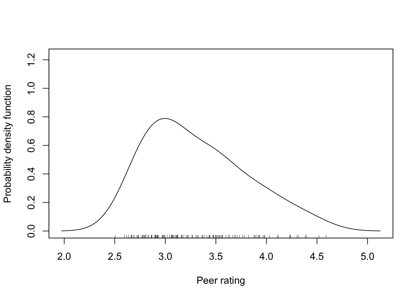
Figure 6.1: Density plot of the outcome variable used in the different models.
Below we show scatterplots of the outcome (peer ratings) versus each of the predictors we are considering in the three scientific models.
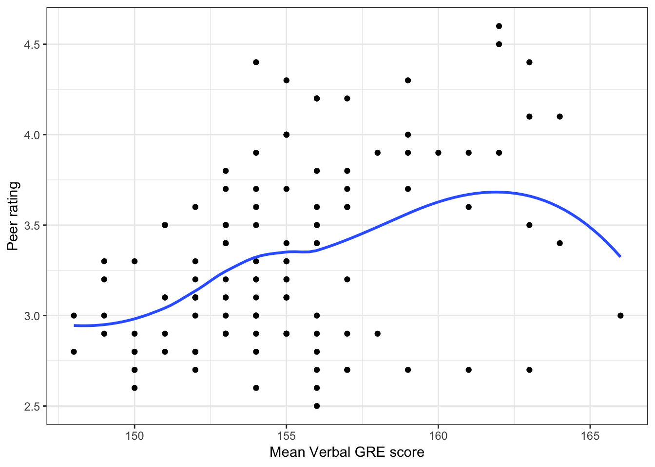
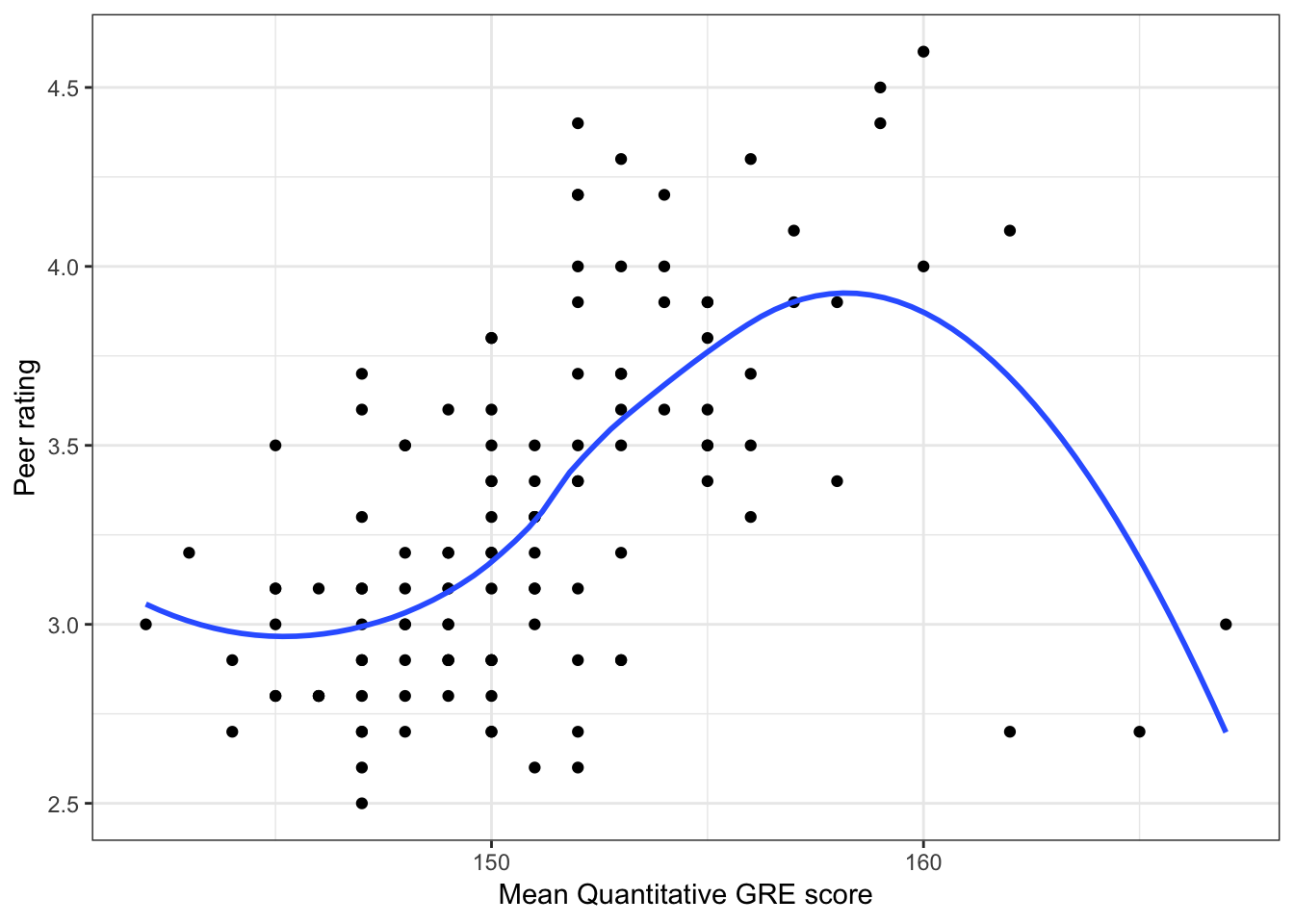
Figure 6.2: Scatterplots of peer ratings versus the student-related factors; verbal and quantitative GRE scores. The loess smoother is also displayed.
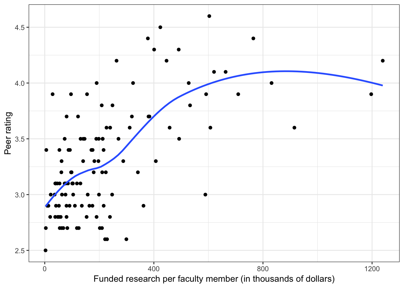
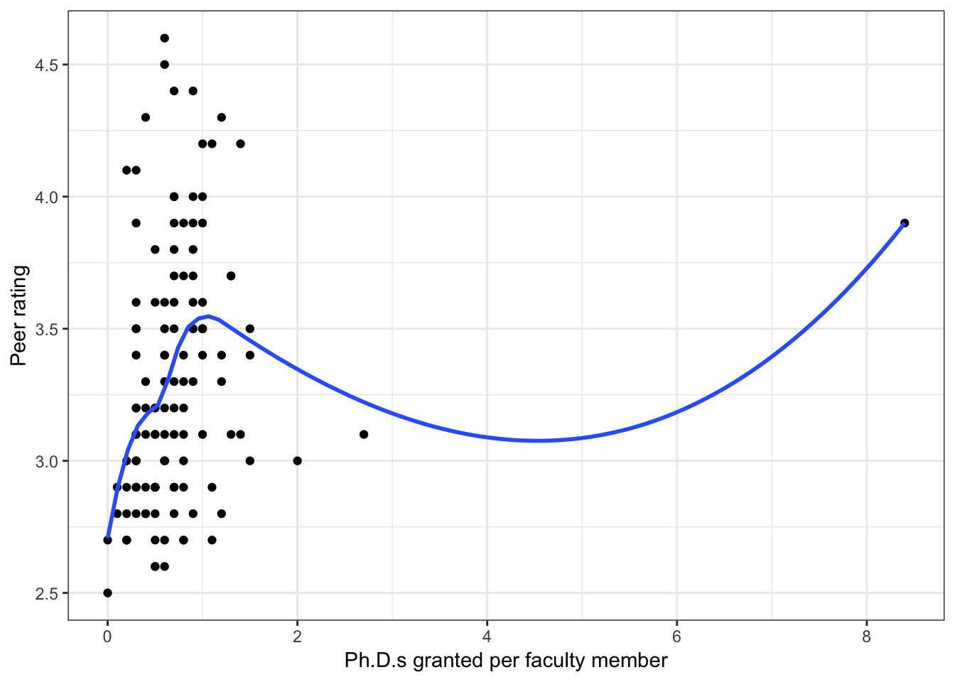
Figure 6.3: Scatterplots of peer ratings versus the faculty-related factors; funded research (per faculty member) and number of Ph.D.s granted (per faculty member). The loess smoother is also displayed.
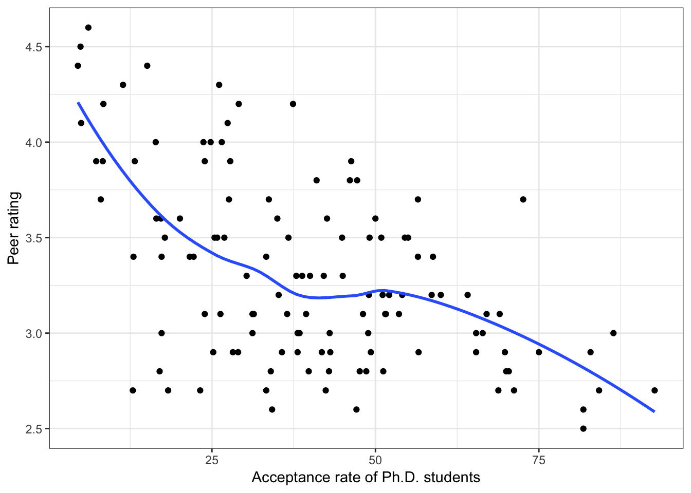
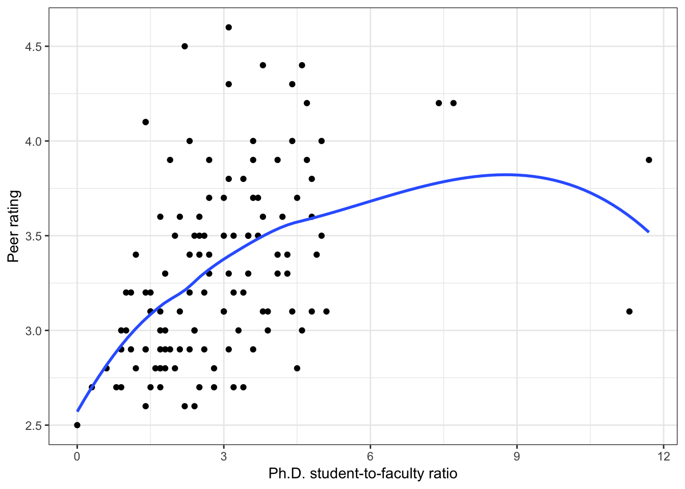
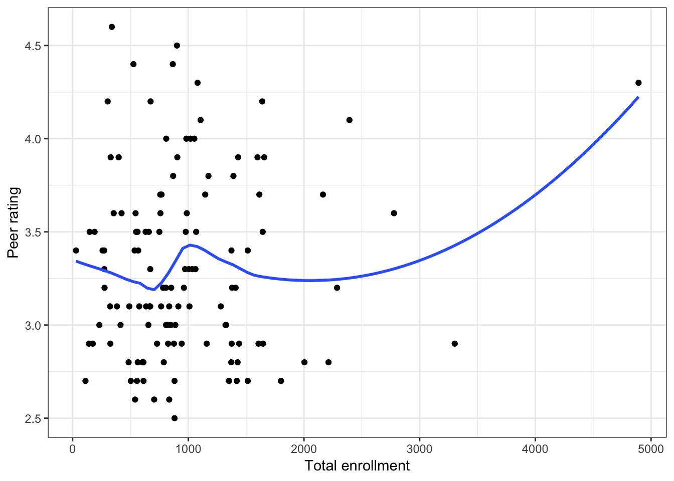
Figure 6.4: Scatterplots of peer ratings versus the institution-related factors; acceptance rate of Ph.D. students, the Ph.D. student-to-faculty ratio, and the size of the program. The loess smoother is also displayed.
Almost all of these plots show curvilinear patterns, some of which can be alleviated by log-transforming the outcome. Remember, log-transforming the outcome will also help with violations of homoskedasticity. Since we want to be able to compare the models at the end of the analysis, we NEED to use the same outcome in each of the models. Given the initial right-skewed nature of the outcome distribution and the evidence from the scatterplots, we will log-transform peer ratings and use that outcome in each model we fit.
# Create log-transformed peer ratings
educ = educ %>%
  mutate(
    Lpeer = log(peer)
    )
6.2.2 Building the Student-Related Factors Model
To determine which of the student-related factors to include in the model, we will examine the scatterplots of each predictor against the log-transformed peer ratings and also examine the correlation matrix of the outcome and student-related predictors.
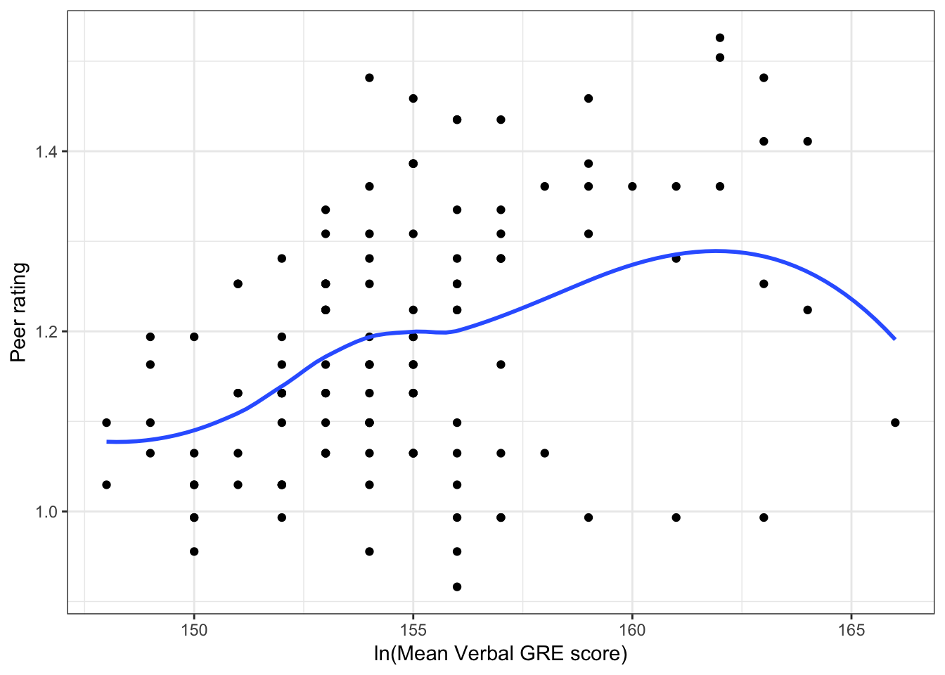
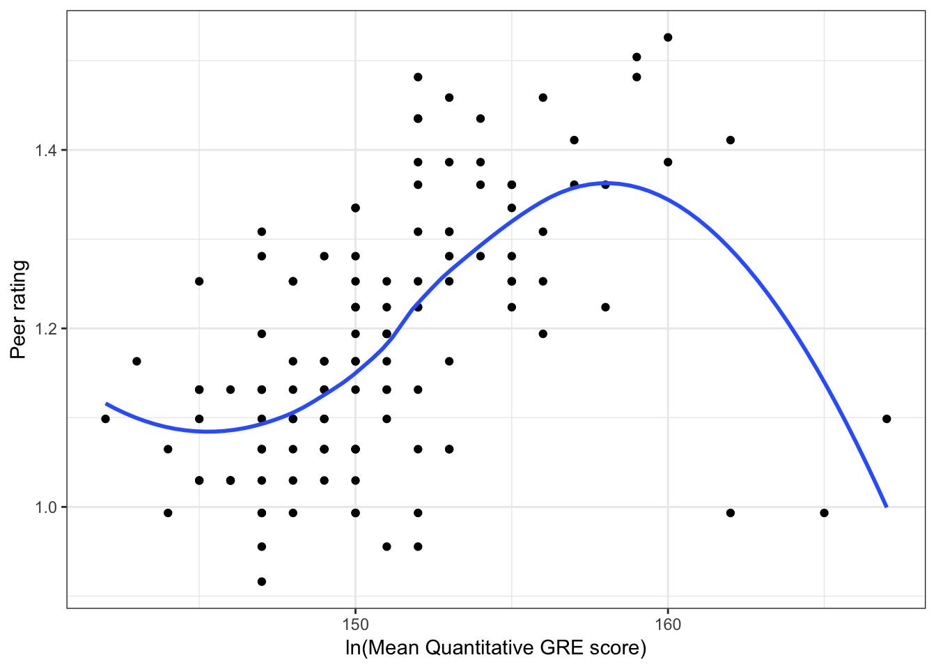
Figure 6.5: Scatterplots of the log-transformed peer ratings versus the student-related factors; verbal and quantitative GRE scores. The loess smoother is also displayed.
educ %>%
  select(Lpeer, gre_verbal, gre_quant) %>%
  correlate()
# A tibble: 3 x 4
rowname Lpeer gre_verbal gre_quant
<chr> <dbl> <dbl> <dbl>
1 Lpeer NA 0.408 0.478
2 gre_verbal 0.408 NA 0.808
3 gre_quant 0.478 0.808 NA Not surprisingly, the mean GRE verbal and GRE quantitative scores are highly correlated. Since including highly correlated predictors in a model can lead to unstable estimates, we will drop one of the predictors from the model. Empirically, the quantitative GRE scores seem more highly correlated with the outcome, so we will drop the GRE verbal scores from the model.
Focusing on the scatterplot of the GRE quantitative scores, the relationship with the log-transformed peer ratings looks curvilinear (non-monotonic). The empirical relationship seems to change direction twice, indicating that log-transformed peer ratings may be a cubic-function of the quantitative GRE scores.
# Fit cubic model
lm.1 = lm(Lpeer ~ 1 + gre_quant + I(gre_quant^2) + I(gre_quant^3), data = educ)

# Coefficient-level output
tidy(lm.1)
# A tibble: 4 x 5
term estimate std.error statistic p.value
<chr> <dbl> <dbl> <dbl> <dbl>
1 (Intercept) 780. 176. 4.43 0.0000210
2 gre_quant -15.4 3.43 -4.49 0.0000165
3 I(gre_quant^2) 0.102 0.0223 4.55 0.0000129
4 I(gre_quant^3) -0.000223 0.0000483 -4.61 0.0000102# Obtain residuals
out_1 = augment(lm.1)
# Examine residuals
sm.density(out_1$.std.resid, xlab = "Standardized residuals", model = "normal")
ggplot(data = out_1, aes(x = .fitted, y = .std.resid)) +
geom_point() +
geom_hline(yintercept = 0) +
theme_bw() +
xlab("Fitted values") +
ylab("Standardized residuals")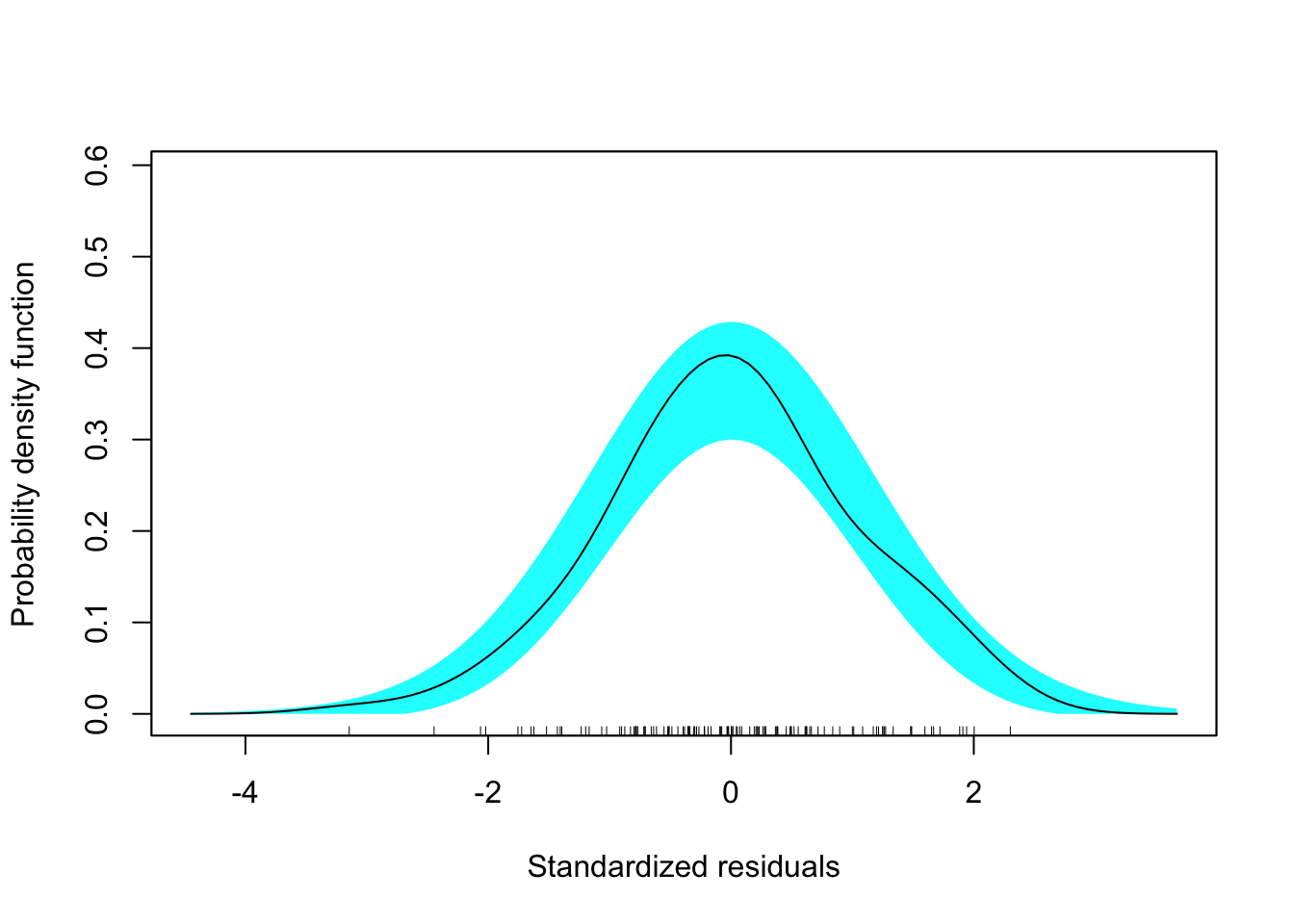

Figure 6.6: Residual plots for the fitted model using the student-related factors.
6.2.3 Building the Faculty-Related Factors Model
To determine which of the faculty-related factors to include in the model, we will examine the scatterplots of each predictor against the log-transformed peer ratings and also examine the correlation matrix of the outcome and faculty-related predictors.
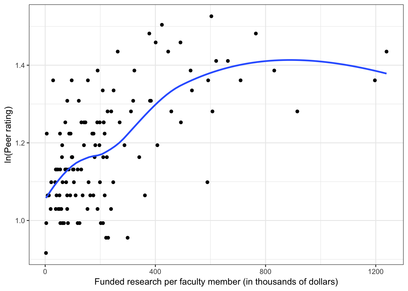
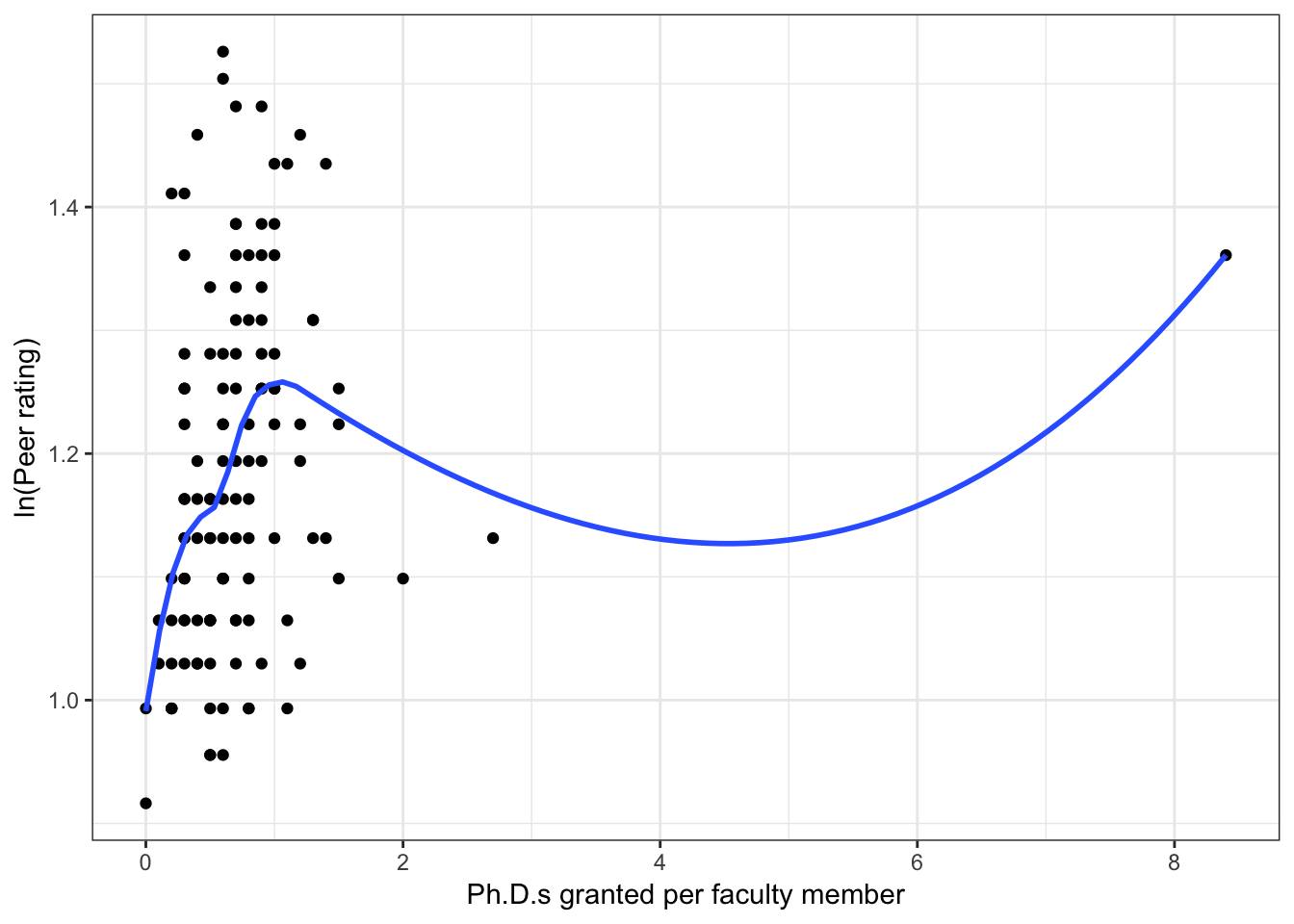
Figure 6.7: Scatterplots of log-transformed peer ratings versus the faculty-related factors; funded research (per faculty member) and number of Ph.D.s granted (per faculty member). The loess smoother is also displayed.
educ %>%
  select(Lpeer, funded_research_per_faculty, phd_granted_per_faculty) %>%
  correlate()
# A tibble: 3 x 4
rowname Lpeer funded_research_per_fa… phd_granted_per_fac…
<chr> <dbl> <dbl> <dbl>
1 Lpeer NA 0.597 0.217
2 funded_research_per_… 0.597 NA 0.403
3 phd_granted_per_facu… 0.217 0.403 NA The two predictors are moderately correlated with each other and both are correlated with the outcome. The scatterplot of peer ratings versus funded research suggest a monotonic curvilinear relationship. The Rule of the Bulge indicates that log-transforming the predictor may help linearize this relationship. The scatterplot of peer ratings versus number of Ph.D.s granted suggests that the distribution of the predictor is right-skewed with a potential outlying observation. This relationship may also benefit from log-transforming the predictor.
Before log-transforming these predictors, it is a good idea to check the distributions for zero or negative values.
educ %>%
  select(funded_research_per_faculty, phd_granted_per_faculty) %>%
  summary()
funded_research_per_faculty phd_granted_per_faculty
Min. : 2.9 Min. :0.000
1st Qu.: 77.8 1st Qu.:0.400
Median : 160.6 Median :0.650
Mean : 228.8 Mean :0.758
3rd Qu.: 283.4 3rd Qu.:0.900
Max. :1239.1 Max. :8.400 The summary values for the phd_granted_per_faculty predictor indicates that there are some schools that have a value of 0 for this predictor and that 0 is the smallest value. Before we transform using a log-transformation, we need to make it so the smallest value in the predictor is 1, since the log of 0 (and any negative values) is undefined. To do this we will add some number (in our case 1) to each value for phd_granted_per_faculty prior to taking the log.
#Create log of the faculty-related predictors
educ = educ %>%
  mutate(
    Lfunded_research_per_faculty = log(funded_research_per_faculty),
    Lphd_granted_per_faculty = log(phd_granted_per_faculty + 1)
  )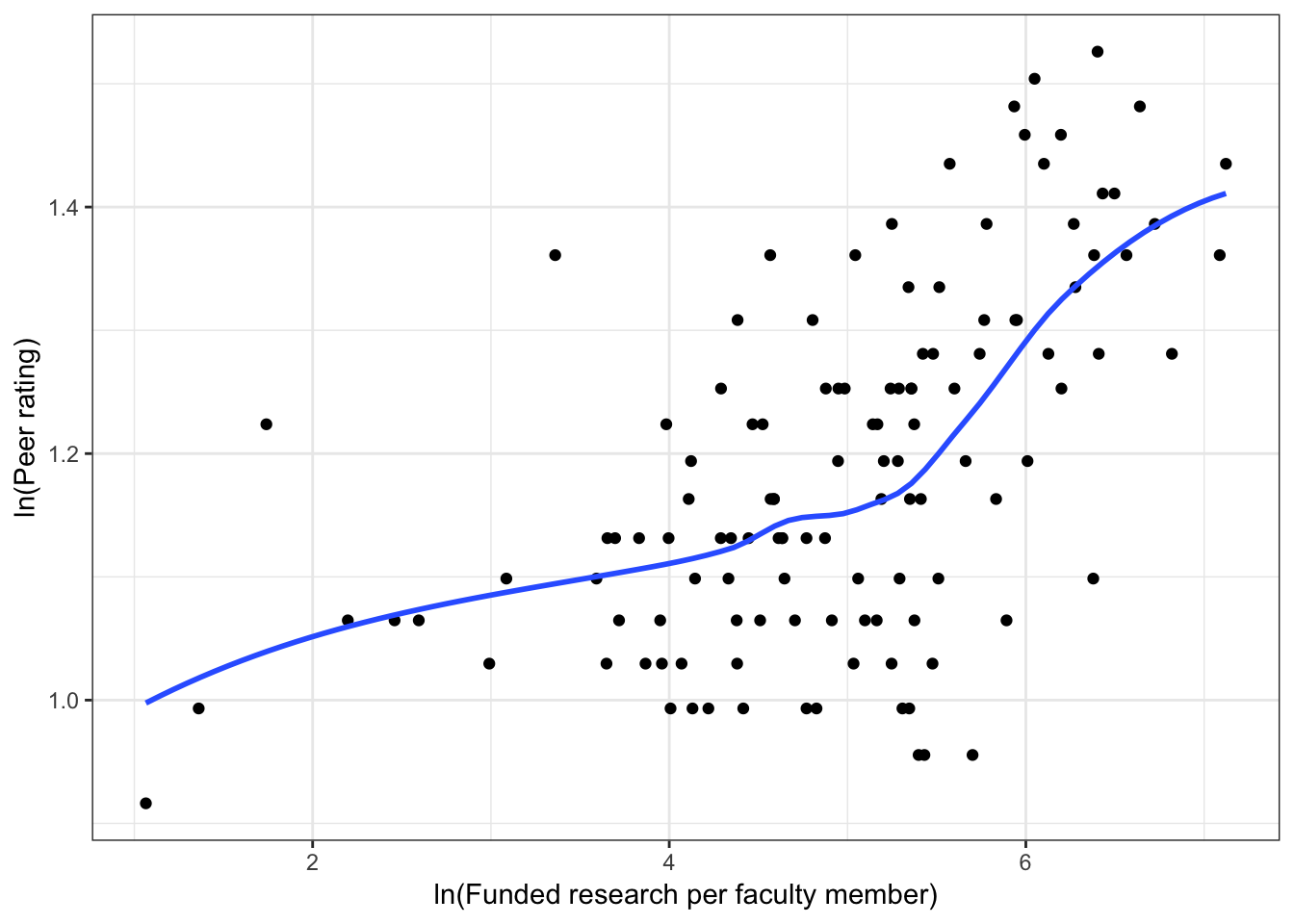
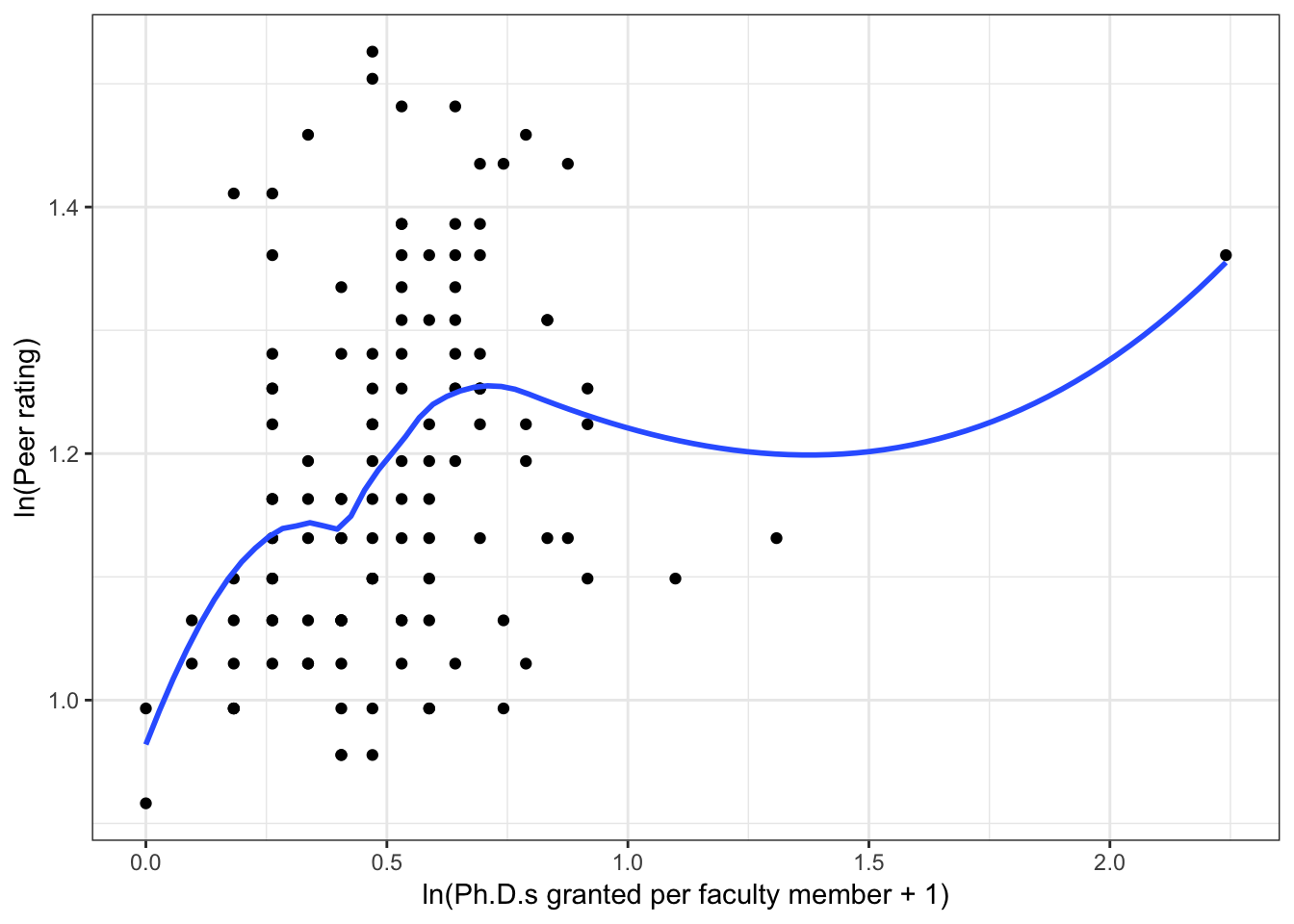
Figure 6.8: Scatterplots of log-transformed peer ratings versus the log-transformed faculty-related factors; funded research (per faculty member) and number of Ph.D.s granted (per faculty member). The loess smoother is also displayed.
Although this helped, it did not “cure” the nonlinearity. We might want to further include a quadratic term for each of the predictors. To evaluate this, we will fit the model that includes the linear and quadratic log-transformed predictors and examine the coefficient-level output and residuals.
# Fit model
lm.2 = lm(Lpeer ~ 1 + Lfunded_research_per_faculty + I(Lfunded_research_per_faculty^2) + Lphd_granted_per_faculty  + I(Lphd_granted_per_faculty^2), data = educ)

# Coefficient-level output
tidy(lm.2)
# A tibble: 5 x 5
term estimate std.error statistic p.value
<chr> <dbl> <dbl> <dbl> <dbl>
1 (Intercept) 1.21 0.106 11.5 6.76e-21
2 Lfunded_research_per_faculty -0.151 0.0509 -2.96 3.70e- 3
3 I(Lfunded_research_per_faculty^2) 0.0238 0.00547 4.35 2.87e- 5
4 Lphd_granted_per_faculty 0.300 0.0948 3.16 1.99e- 3
5 I(Lphd_granted_per_faculty^2) -0.139 0.0503 -2.77 6.58e- 3# Obtain residuals
out_2 = augment(lm.1)
# Examine residuals
sm.density(out_2$.std.resid, xlab = "Standardized residuals", model = "normal")
ggplot(data = out_2, aes(x = .fitted, y = .std.resid)) +
geom_point() +
geom_hline(yintercept = 0) +
theme_bw() +
xlab("Fitted values") +
ylab("Standardized residuals")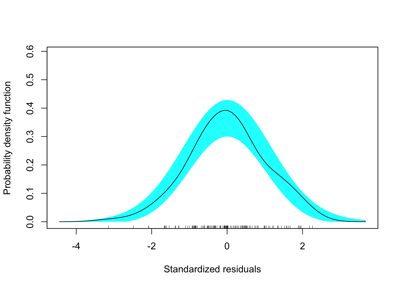
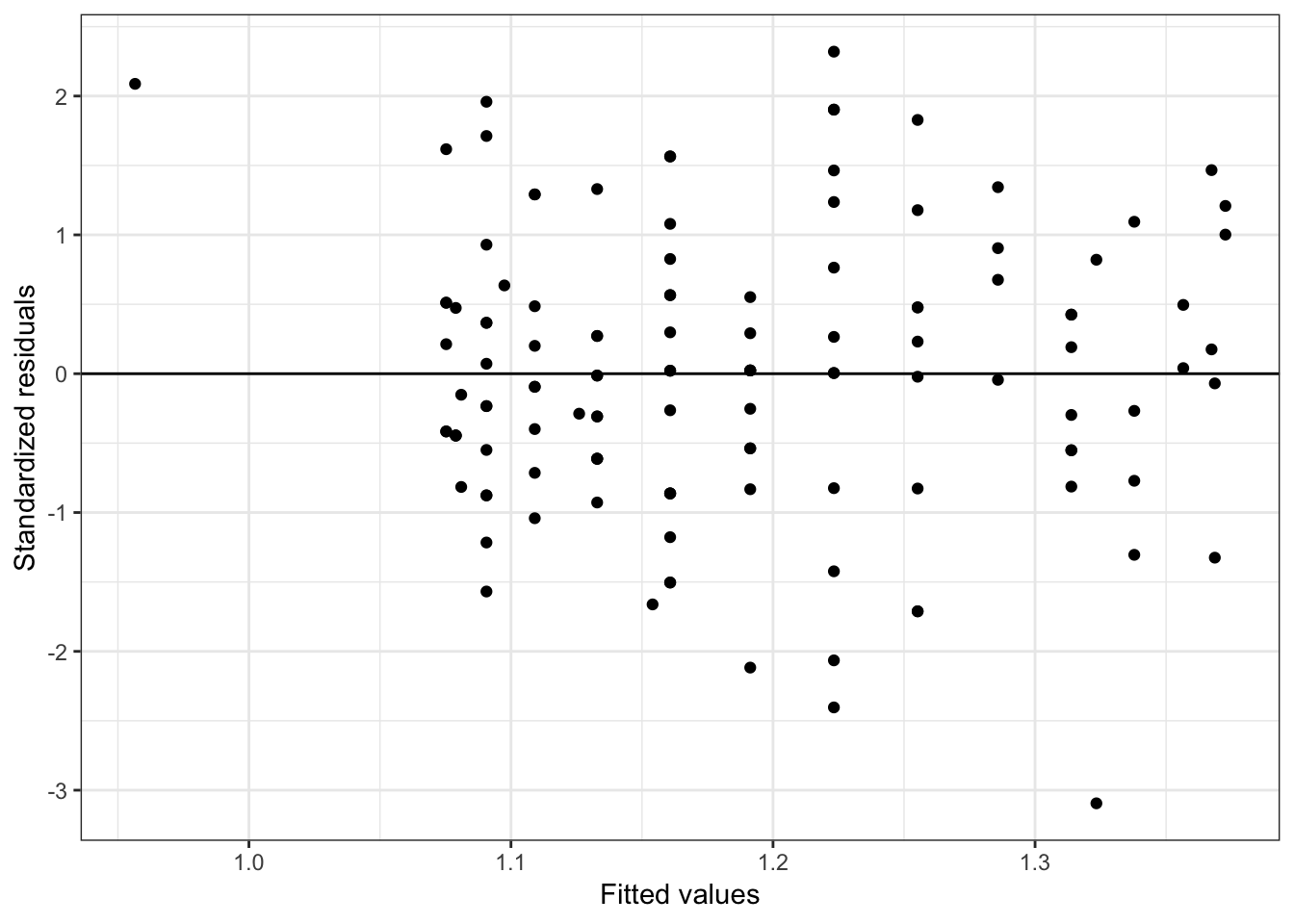
Figure 6.9: Residual plots for the fitted model using the faculty-related factors.
6.2.4 Building the Institution-Related Factors Model
To determine which of the institution-related factors to include in the model, we will examine the scatterplots of each predictor against the log-transformed peer ratings and also examine the correlation matrix of the outcome and institution-related predictors.
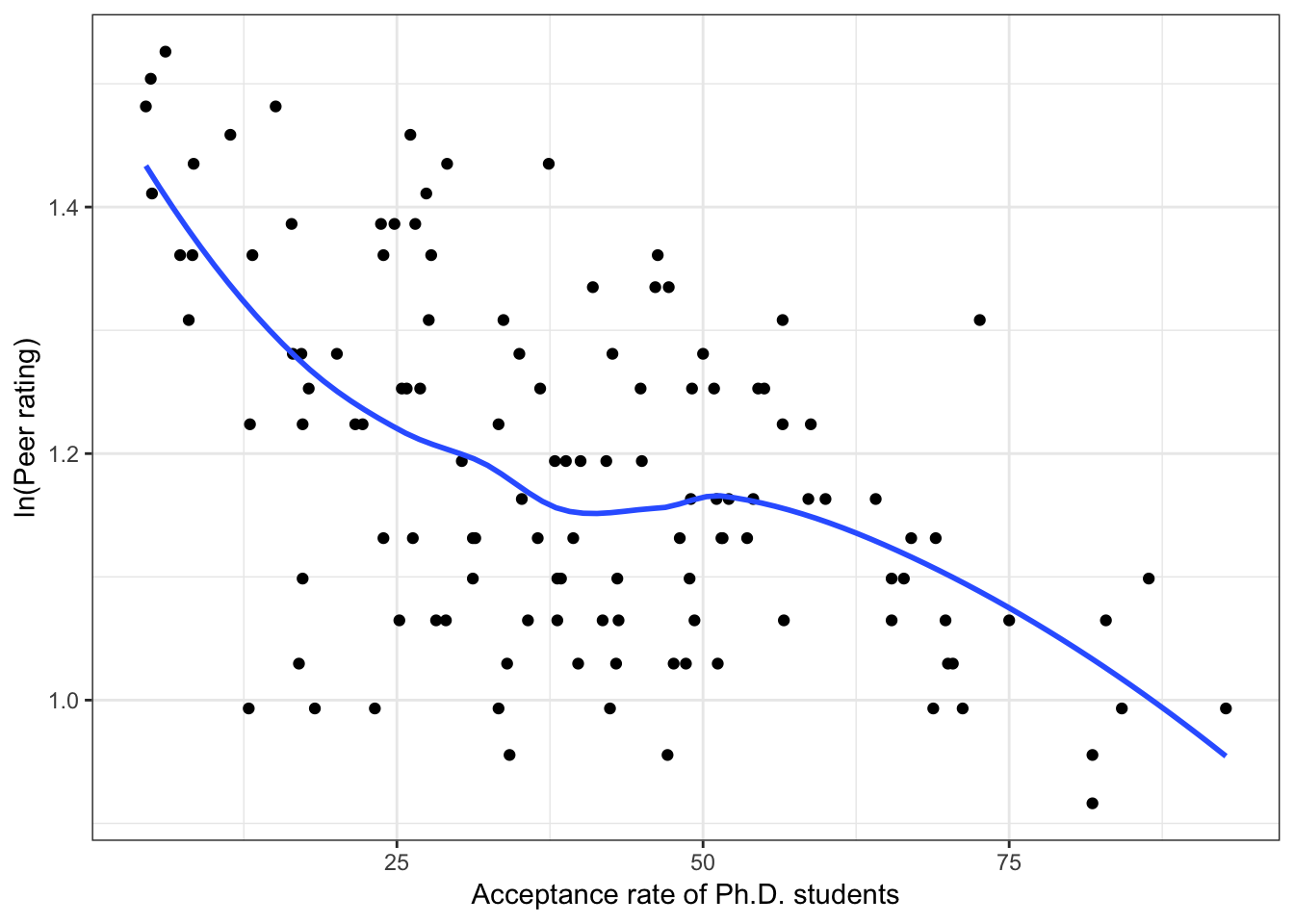
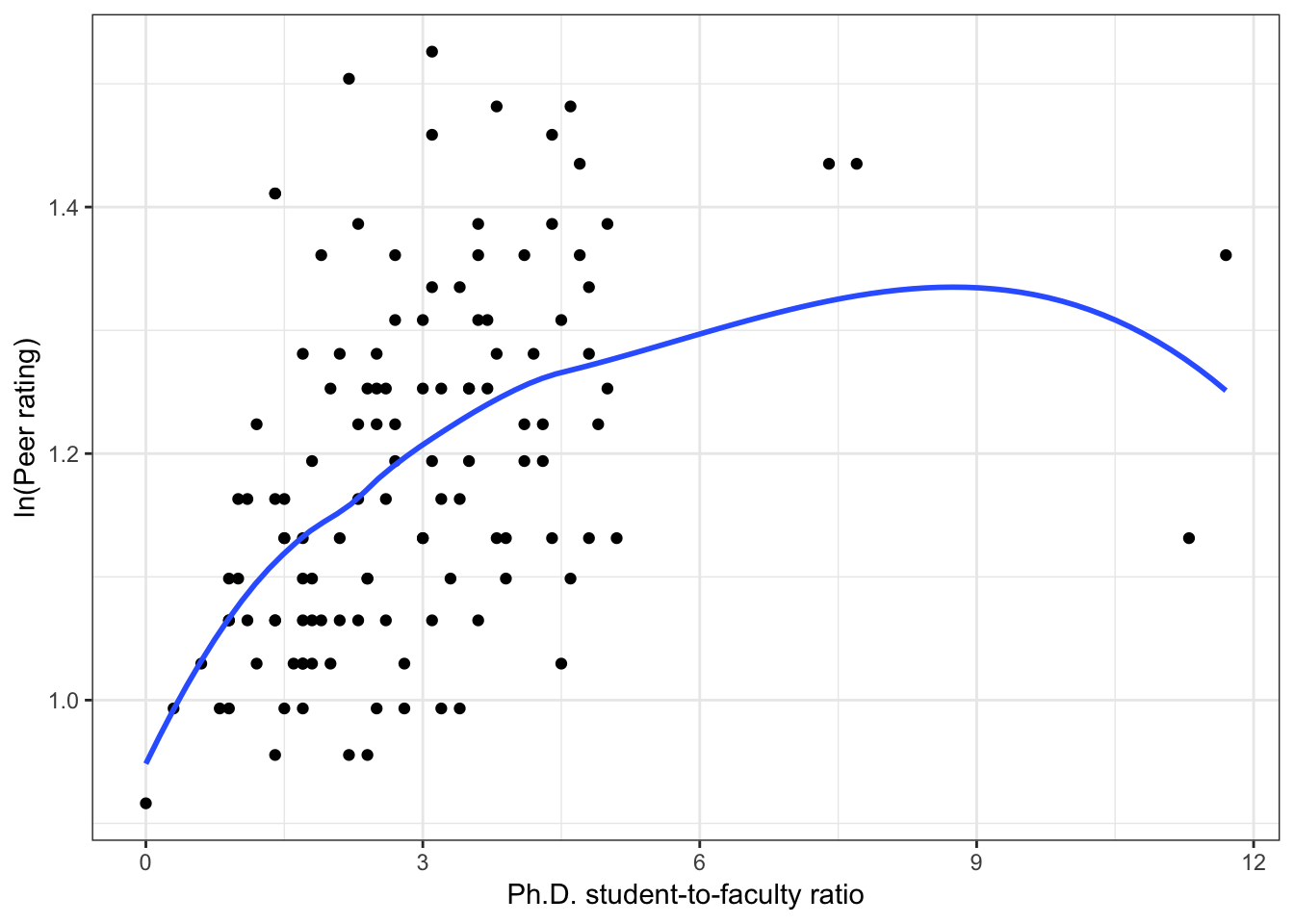
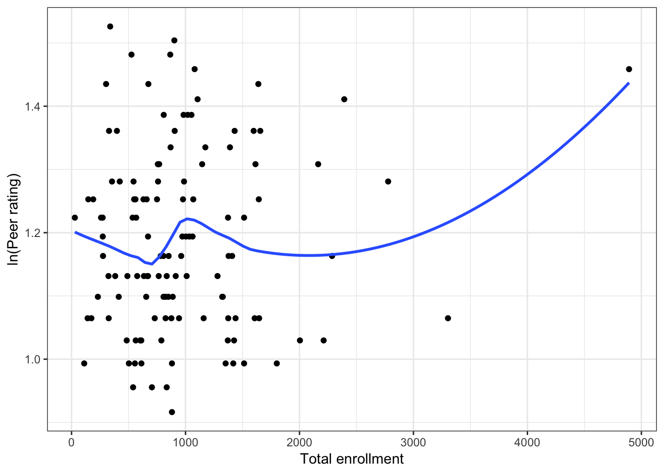
Figure 6.10: Scatterplots of the log-transformed peer ratings versus the institution-related factors; acceptance rate of Ph.D. students, the Ph.D. student-to-faculty ratio, and the size of the program. The loess smoother is also displayed.
educ %>%
  select(Lpeer, doc_accept, phd_student_faculty_ratio, enroll) %>%
  correlate()
# A tibble: 4 x 5
rowname Lpeer doc_accept phd_student_faculty_r… enroll
<chr> <dbl> <dbl> <dbl> <dbl>
1 Lpeer NA -0.534 0.423 0.0964
2 doc_accept -0.534 NA -0.235 -0.0256
3 phd_student_faculty… 0.423 -0.235 NA 0.00450
4 enroll 0.0964 -0.0256 0.00450 NA The three predictors are mostly uncorrelated with each other and all are correlated with the outcome, albeit enrollment is weakly correlated with peer ratings. Two of the three scatterplots suggest curvilinear relationships although with different functional forms—Ph.D. student-to-faculty ratio and total enrollment. The Rule of the Bulge indicates that log-transforming the Ph.D. student-to-faculty ratio predictor, and including quadratic may help linearize this relationship. The scatterplot of peer ratings versus total enrollment suggests that the distribution of the predictor is right-skewed with a potential outlying observations. This relationship may also benefit from log-transforming the predictor. Lastly, it is unclear whether any additional transformation or polynomial terms are necessary for modeling the relationship with doctoral acceptance rate; to double-check this we will also log-transform the total enrollment predictor.
As before, prior to log-transforming any predictors, it is a good idea to check the distributions for zero or negative values.
educ %>%
  select(doc_accept, phd_student_faculty_ratio, enroll) %>%
  summary()
doc_accept phd_student_faculty_ratio enroll
Min. : 4.5 Min. : 0.00 Min. : 29
1st Qu.:25.5 1st Qu.: 1.70 1st Qu.: 562
Median :38.6 Median : 2.70 Median : 842
Mean :40.1 Mean : 2.94 Mean : 970
3rd Qu.:51.6 3rd Qu.: 3.77 3rd Qu.:1312
Max. :92.7 Max. :11.70 Max. :4892 We will need to add one to every value of the phd_student_faculty_ratio predictor (so that the minimum value becomes 1) prior to the log-transformation.
#Create log of the faculty-related predictors
educ = educ %>%
  mutate(
    Ldoc_accept = log(doc_accept),
    Lphd_student_faculty_ratio = log(phd_student_faculty_ratio + 1),
    Lenroll = log(enroll)
  )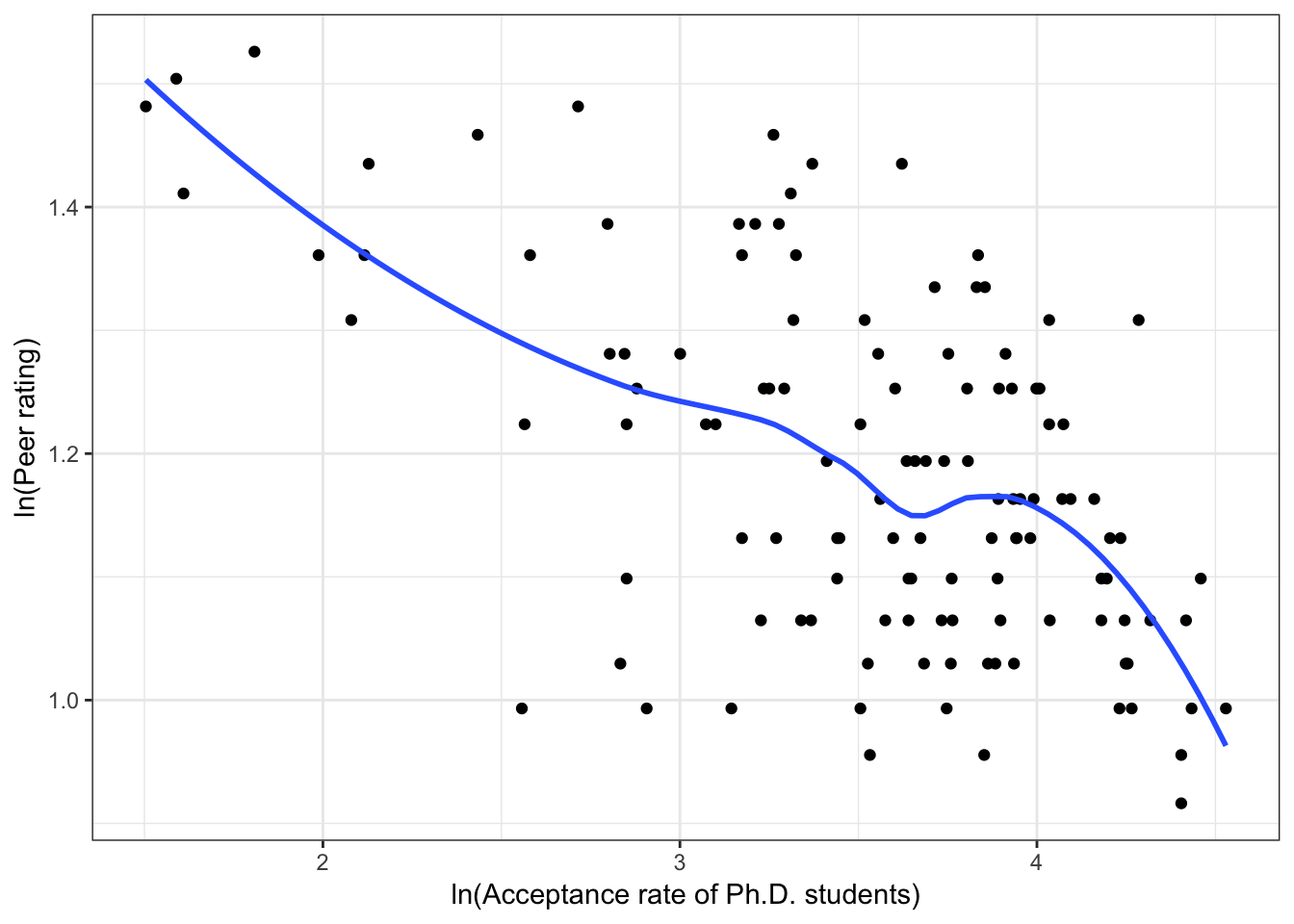
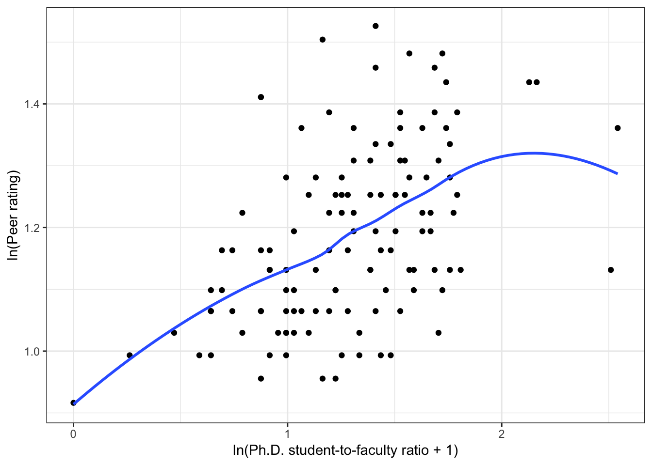
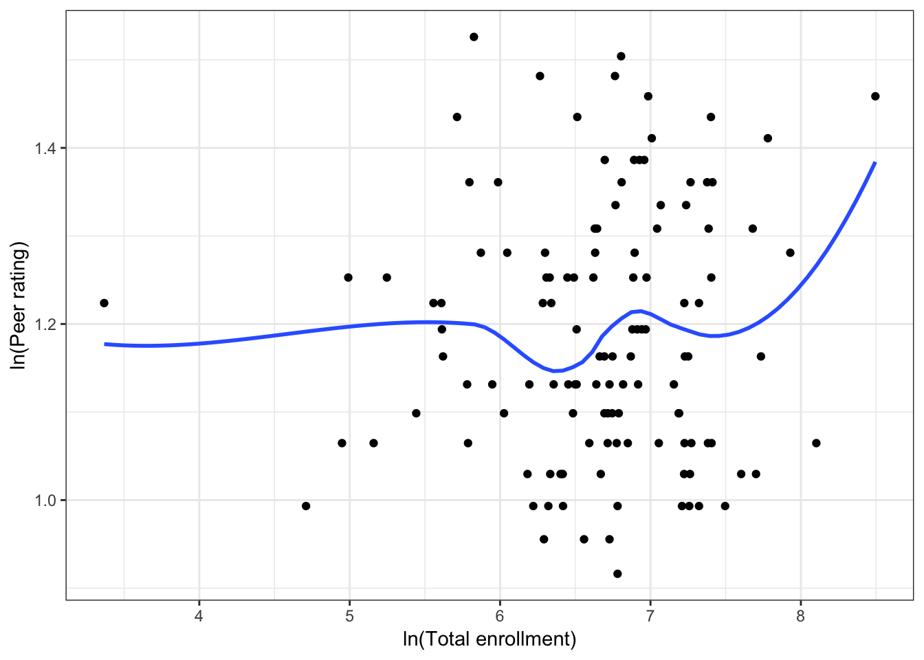
Figure 6.11: Scatterplots of the log-transformed peer ratings versus the log-transformed institution-related factors. The loess smoother is also displayed.
The scatterplots indicate that all three relationships were satisfactorily linearized. After fitting the institution-related factors model we will further examine the coefficient-level output and residuals.
# Fit model
lm.3 = lm(Lpeer ~ 1 + Ldoc_accept + Lenroll + Lphd_student_faculty_ratio, data = educ)

# Coefficient-level output
tidy(lm.3)
# A tibble: 4 x 5
term estimate std.error statistic p.value
<chr> <dbl> <dbl> <dbl> <dbl>
1 (Intercept) 1.31 0.108 12.1 1.96e-22
2 Ldoc_accept -0.109 0.0156 -6.97 1.95e-10
3 Lenroll 0.0145 0.0136 1.07 2.87e- 1
4 Lphd_student_faculty_ratio 0.129 0.0247 5.20 8.42e- 7# Obtain residuals
out_3 = augment(lm.3)
# Examine residuals
sm.density(out_3$.std.resid, xlab = "Standardized residuals", model = "normal")
ggplot(data = out_3, aes(x = .fitted, y = .std.resid)) +
geom_point() +
geom_hline(yintercept = 0) +
theme_bw() +
xlab("Fitted values") +
ylab("Standardized residuals")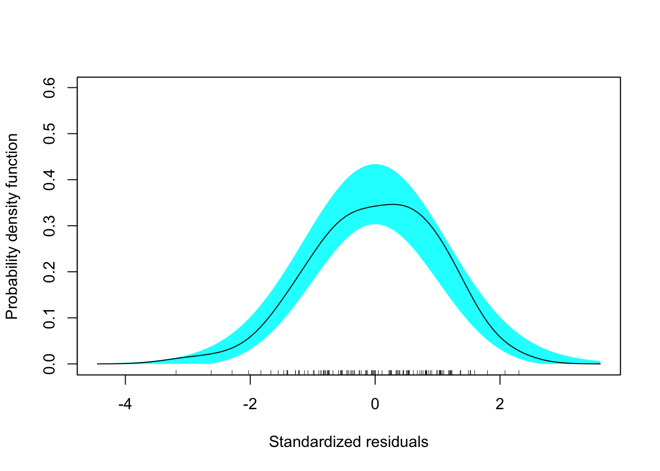
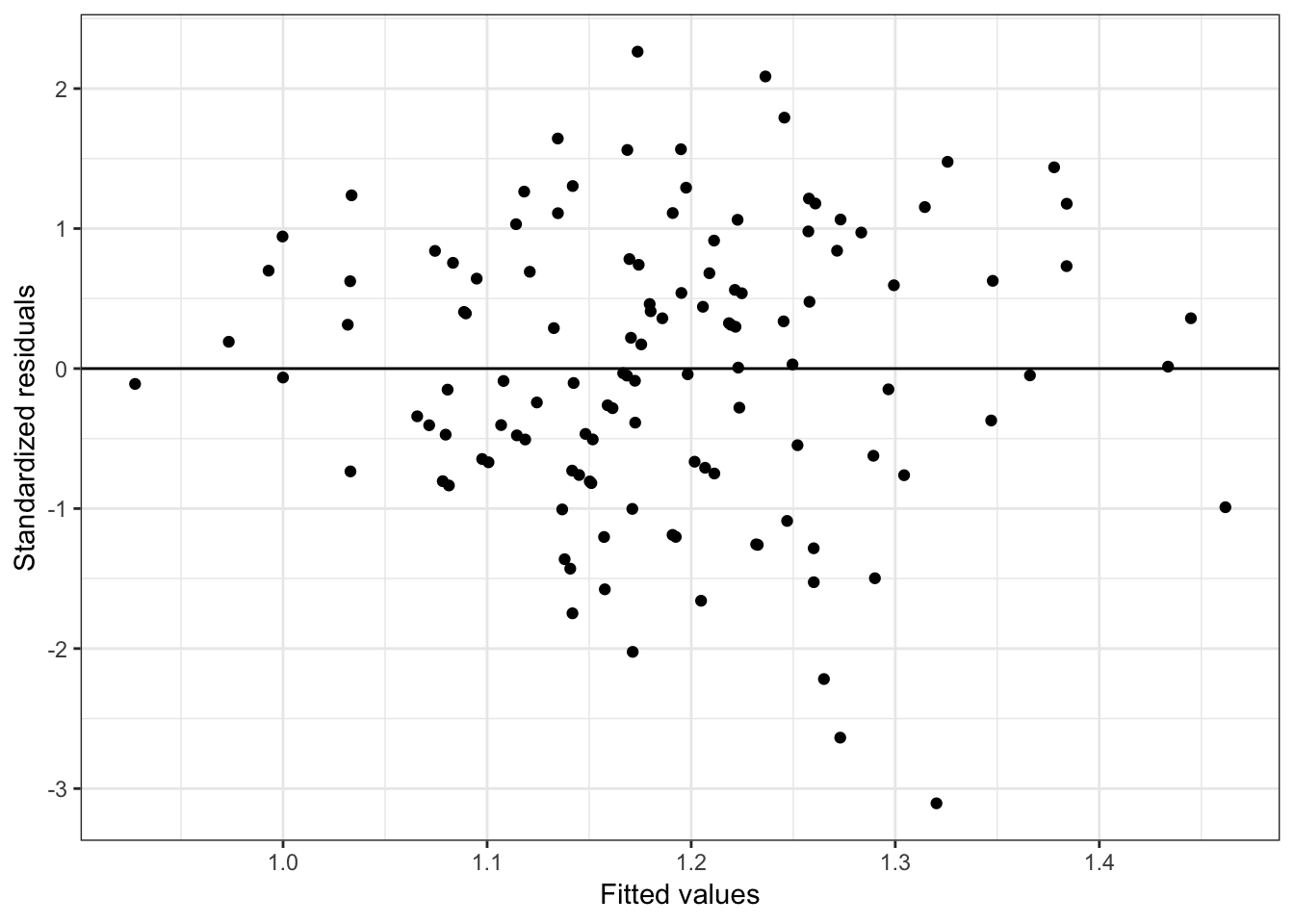
Figure 6.12: Residual plots for the fitted model using the institution-related factors.
The coefficient-level output indicates that the log-transformed enrollment predictor may be unnecessary (\(p=0.287\)). We will fit another model that omits this predictor, but we will also retain this initial model as it was suggested from the scientific research.
# Fit model
lm.4 = lm(Lpeer ~ 1 + Ldoc_accept + Lphd_student_faculty_ratio, data = educ)

# Coefficient-level output
tidy(lm.4)
# A tibble: 3 x 5
term estimate std.error statistic p.value
<chr> <dbl> <dbl> <dbl> <dbl>
1 (Intercept) 1.40 0.0704 19.8 1.56e-39
2 Ldoc_accept -0.107 0.0155 -6.89 2.81e-10
3 Lphd_student_faculty_ratio 0.131 0.0247 5.31 5.28e- 7# Obtain residuals
out_4 = augment(lm.4)
# Examine residuals
sm.density(out_4$.std.resid, xlab = "Standardized residuals", model = "normal")
ggplot(data = out_4, aes(x = .fitted, y = .std.resid)) +
geom_point() +
geom_hline(yintercept = 0) +
theme_bw() +
xlab("Fitted values") +
ylab("Standardized residuals")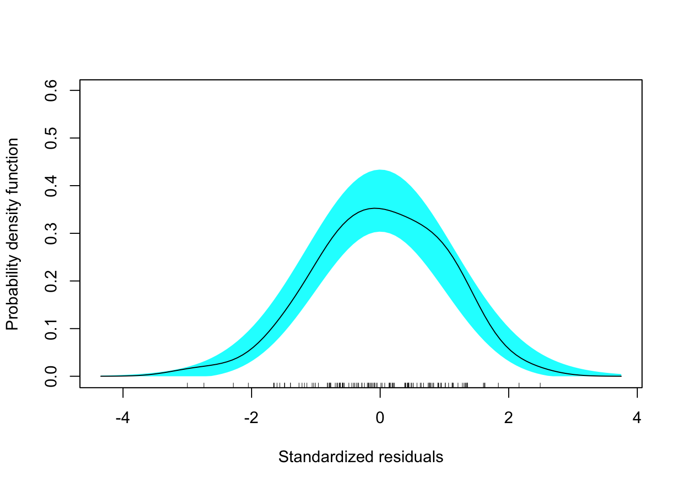
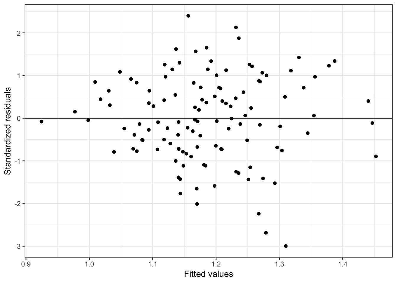
Figure 6.13: Residual plots for the fitted model using the institution-related factors (enrollment omitted).
6.3 Candidate Statistical Models
Now that we have settled on the functional form for each of the three proposed models, we can write out the statistical models associated with the scientific hypotheses. These models using regression notation are:
- M1: \(\mathrm{Peer~Rating}_i = \beta_0 + \beta_1(\mathrm{GREQ}_i) + \beta_2(\mathrm{GREQ}^2_i) + \beta_3(\mathrm{GREQ}^3_i) + \epsilon_i\)
- M2: \(\mathrm{Peer~Rating}_i = \beta_0 + \beta_1(\mathrm{Funded~research}_i) + \beta_2(\mathrm{Funded~research}^2_i) + \beta_3(\mathrm{PhDs~granted}_i) + \beta_4(\mathrm{PhDs~granted}^2_i) + \epsilon_i\)
- M3: \(\mathrm{Peer~Rating}_i = \beta_0 + \beta_1(\mathrm{PhD~acceptance~rate}_i) + \beta_2(\mathrm{PhD~student\mbox{-}to\mbox{-}faculty~ratio}_i) + \beta_3(\mathrm{Enrollment}_i) + \epsilon_i\)
where peer rating, funded research, Ph.D.s granted, Ph.D. acceptance rate, enrollment, and Ph.D. student-to-faculty ratio have all been log-transformed. We will also consider a fourth model that omits enrollment from the institution-related factors model.
- M4: \(\mathrm{Peer~Rating}_i = \beta_0 + \beta_1(\mathrm{PhD~acceptance~rate}_i) + \beta_2(\mathrm{PhD~student\mbox{-}to\mbox{-}faculty~ratio}_i) + \epsilon_i\)
6.4 Log-Likelihood
Recall that the likelihood gives us the probability of a particular model given a set of data and assumptions about the model, and that the log-likelihood is just a mathematically convenient transformation of the likelihood. Log-likelihood values from different models can be compared, so long as:
- The exact same data is used to fit the models,
- The exact same outcome is used to fit the models, and
- The assumptions underlying the likelihood (independence, distributional assumptions) are met.
In all four models we are using the same data set and outcome, and the assumptions seem reasonably tenable for each of the four fitted candidate models. This suggests that the likelihood (or log-likelihood) can provide some evidence as to which of the four candidate models is most probable. Below we compute the log-likelihood values for each of the four candidate models.
logLik(lm.1)'log Lik.' 95.88 (df=5)logLik(lm.2)'log Lik.' 98.25 (df=6)logLik(lm.3)'log Lik.' 101.4 (df=5)logLik(lm.4)'log Lik.' 100.8 (df=4)Note that the log-likelihood values are also available from the glance() function’s output (in the logLik column).
glance(lm.1)# A tibble: 1 x 11
r.squared adj.r.squared sigma statistic p.value df logLik AIC BIC
<dbl> <dbl> <dbl> <dbl> <dbl> <int> <dbl> <dbl> <dbl>
1 0.409 0.394 0.112 27.2 1.96e-13 4 95.9 -182. -168.
# … with 2 more variables: deviance <dbl>, df.residual <int>These values suggest that the model with the highest probability given the data and set of assumptions is Model 3; it has the highest log-likelihood value.
6.5 Deviance: An Alternative Fit Value
It is common to multiply the log-likelihood values by \(-2\). This is called the deviance. Deviance is a measure of model-data error, so when evaluating deviance values, lower is better. (The square brackets in the syntax grab the log-likelihood value from the logLik() output.)
-2 * logLik(lm.1)[1] #Model 1[1] -191.8-2 * logLik(lm.2)[1] #Model 2[1] -196.5-2 * logLik(lm.3)[1] #Model 3[1] -202.8-2 * logLik(lm.4)[1] #Model 4[1] -201.7Here, the model that produces the lowest amount of model-data error is Model 3; it has the lowest deviance value. Since the deviance just multiplies the log-likelihood values by a constant, it produces the same rank ordering of the candidate models. Thus, whether you evaluate using the likelihood, the log-likelihood, or the deviance, you will end up with the same ordering of candidate models. Using deviance, however, has the advantages of having a direct relationship to model error, so it is more interpretable. It is also more closely aligned with other model measures associated with error that we commonly use (e.g., SSE, \(R^2\)).
6.6 Akiake’s Information Criteria (AIC)
Remember that lower values of deviance indicate the model (as defined via the set of parameters) is more likely (lower model-data error) given the data and set of assumptions. However, in practice we cannot directly compare the deviances since the models include a different number of parameters. It was not coincidence that our most probable candidate model also had the highest number of predictors.
To account for this, we will add a penalty term to the deviance based on the number of parameters estimated in the model. This penalty-adjusted value is called Akiake’s Information Criteria (AIC).
\[ AIC = \mathrm{Deviance} + 2(k) \]
where \(k\) is the number of parameters being estimated in the model (including the intercept and RMSE). The AIC adjusts the deviance based on the complexity of the model. Note that the value for \(k\) is given as df in the logLik() output. For our four models, the df values are:
- M1: 5 df (\(\hat\beta_0\), \(\hat\beta_1\), \(\hat\beta_2\), \(\hat\beta_3\), RMSE)
- M2: 6 df (\(\hat\beta_0\), \(\hat\beta_1\), \(\hat\beta_2\), \(\hat\beta_3\), \(\hat\beta_4\), RMSE)
- M3: 5 df (\(\hat\beta_0\), \(\hat\beta_1\), \(\hat\beta_2\), \(\hat\beta_3\), RMSE)
- M4: 4 df (\(\hat\beta_0\), \(\hat\beta_1\), \(\hat\beta_2\), RMSE)
Just as with the deviance, smaller AIC values indicate a more likely model.
-2 * logLik(lm.1)[1] + 2*5 #Model 1[1] -181.8-2 * logLik(lm.2)[1] + 2*6 #Model 2[1] -184.5-2 * logLik(lm.3)[1] + 2*5 #Model 3[1] -192.8-2 * logLik(lm.4)[1] + 2*4 #Model 4[1] -193.7Arranging these, we find that Model 4 (AIC = \(-193.7\)) is the most likely candidate model given the data and candidate set of models. This leads us to adopt Model 4 (the reduced model) over Model 3 (the full model) for the institution-related factors model.
We can also compute the AIC via the AIC() function.
# Compute AIC value for Model 4
AIC(lm.4)
[1] -193.7Lastly, we note that the AIC value is produced as a column in the model-level output. (Note that the df column from glance() does NOT give the number of model parameters.)
# Model-level output for Model 4
glance(lm.4)
# A tibble: 1 x 11
r.squared adj.r.squared sigma statistic p.value df logLik AIC BIC
<dbl> <dbl> <dbl> <dbl> <dbl> <int> <dbl> <dbl> <dbl>
1 0.455 0.446 0.107 49.6 2.12e-16 3 101. -194. -182.
# … with 2 more variables: deviance <dbl>, df.residual <int>6.7 Empirical Support for Hypotheses
Because the models are proxies for the scientific working hypotheses, the AIC ends up being a measure of empirical support for any particular hypothesis—after all, it takes into account the data (empirical evidence) and model complexity. In practice, we can use the AIC to rank order the models, which results in a rank ordering of the scientific working hypotheses based on the empirical support for each. Ranked in order of empirical support, the three scientific working hypotheses are:
- Peer ratings are attributable to institution-related factors. This hypothesis has the most empirical support of the three working hypotheses, given the data and other candidate models.
- Peer ratings are attributable to faculty-related factors.
- Peer ratings are attributable to student-related factors. This hypothesis has the least amount of empirical support of the three working hypotheses, given the data and other candidate models.
It is important to remember that the phrase “given the data and other candidate models” is highly important. Using AIC to rank order the models results in a relative ranking of the models. It is not able to rank any hypotheses that you didn’t consider as part of the candidate set of scientific working hypotheses. Moreover, the AIC is a direct function of the likelihood which is based on the actual model fitted as a proxy for the scientific working hypothesis. If the predictors used in any of the models had been different, it would lead to different likelihood and AIC values, and potentially a different rank ordering of the hypotheses.
As an example, consider if we had not done any exploration of the model’s functional form, but instead had just included the linear main-effects for each model.
# Fit models
lm.1 = lm(peer ~ 1 + gre_quant + gre_verbal, data = educ)
lm.2 = lm(peer ~ 1 + funded_research_per_faculty + phd_granted_per_faculty, data = educ)
lm.3 = lm(peer ~ 1 + doc_accept + enroll + phd_student_faculty_ratio, data = educ)

# Compute AIC values
AIC(lm.1)
[1] 144.8AIC(lm.2)[1] 121.6AIC(lm.3)[1] 121In this example, the rank-ordering of hypotheses ended up being the same, but the actual AIC values were quite different. This will play an even bigger role in the next set of notes where we compare the size of the different AIC values to look at how much more empirical support one hypothesis has versus another.
Finally, it is important to mention that philosophically, the use of information-criteria for model selection is not compatible with using \(p\)-values for variable selection. As an example consider Model 3 and Model 4:
\[ \begin{split} \mathbf{Model~3:~} & \mathrm{Peer~Rating}_i = \beta_0 + \beta_1(\mathrm{PhD~acceptance~rate}_i) + \beta_2(\mathrm{PhD~student\mbox{-}to\mbox{-}faculty~ratio}_i) + \beta_3(\mathrm{Enrollment}_i) + \epsilon_i \\ \mathbf{Model~4:~} & \mathrm{Peer~Rating}_i = \beta_0 + \beta_1(\mathrm{PhD~acceptance~rate}_i) + \beta_2(\mathrm{PhD~student\mbox{-}to\mbox{-}faculty~ratio}_i) + \epsilon_i \end{split} \]
Using \(p\)-values for variable selection, we would have fitted Model 3, found that the \(p\)-value associated with the enrollment coefficient was non-significant, and dropped enrollment from the model. Using the AIC values however, we also dropped enrollment from the model as the AIC value for Model 4 was smaller than the AIC value for Model 3.
Although in this case we came to the same conclusion, these methods are based on two very different philosophies of measuring statistical evidence. The \(p\)-value is a measure of how rare an observed statistic (e.g., \(\hat\beta_k\), \(t\)-value) is under the null hypothesis. The AIC, on the other hand, is a measure of the model-data compatibility accounting for the complexity of the model.
In general, the use of \(p\)-values is not compatible with the use of model-level selection methods such as information criteria; see Anderson (2008) for more detail. Because of this, it is typical to not even report \(p\)-values when carrying out this type of analysis.
References
Anderson, D. R. (2008). Model based inference in the life sciences: A primer on evidence. New York: Springer.