Unit 8: Introduction to Mixed-Effects Models
In this set of notes, you will learn the conceptual ideas behind linear mixed-effects models, also called multilevel models or hierarchical linear models.
Preparation
Before class you will need to read the Relational data chapter from following:
- Grolemund, G., & Wickham, H. (2017). R for Data Science: Visualize, model, transform, tidy, and import data. **. Sebastopol, CA: O’Reilly.
Focus on the information on mutating joins.
8.1 Dataset and Research Question
In this set of notes, we will use data from two files, the netherlands-students.csv file and the netherlands-schools.csv files (see the data codebook here). These data include student- and school-level attributes, respectively, for \(n_i=2287\) 8th-grade students in the Netherlands.
# Load libraries
library(broom)
library(dplyr)
library(ggplot2)
library(lme4) #for fitting mixed-effects models
library(readr)
library(sm)

# Read in student-level data
student_data = read_csv(file = "~/Documents/github/epsy-8252/data/netherlands-students.csv")
head(student_data)
# A tibble: 6 x 8
student_id school_id language_pre language_post ses verbal_iq female
<dbl> <dbl> <dbl> <dbl> <dbl> <dbl> <dbl>
1 17001 1 36 46 23 3.17 0
2 17002 1 36 45 10 2.67 0
3 17003 1 33 33 15 -2.33 0
4 17004 1 29 46 23 -0.834 0
5 17005 1 19 20 10 -3.83 0
6 17006 1 22 30 10 -2.33 0
# … with 1 more variable: minority <dbl># Read in school-level data
school_data = read_csv(file = "~/Documents/github/epsy-8252/data/netherlands-schools.csv")
head(school_data)# A tibble: 6 x 6
school_id school_type public school_ses school_verbal_iq school_minority
<dbl> <chr> <dbl> <dbl> <dbl> <dbl>
1 15 Catholic 0 18 -0.334 25
2 36 Catholic 0 20 -0.138 0
3 40 Catholic 0 23 0.652 0
4 42 Catholic 0 24 -0.0126 0
5 44 Catholic 0 14 -0.634 20
6 47 Catholic 0 11 -3.52 8We will use these data to explore the question of whether verbal IQ scores predict variation in post-test language scores.
8.2 Join the Student- and Classroom-Level Data
Before analyzing the data, we need to join, or merge, the two datasets together. To do this, we will use the left_join() function from the dplyr package. dplyr includes six different join functions. You can read about several different join functions here.
joined_data = left_join(student_data, school_data, by = "school_id")
head(joined_data)
# A tibble: 6 x 13
student_id school_id language_pre language_post ses verbal_iq female
<dbl> <dbl> <dbl> <dbl> <dbl> <dbl> <dbl>
1 17001 1 36 46 23 3.17 0
2 17002 1 36 45 10 2.67 0
3 17003 1 33 33 15 -2.33 0
4 17004 1 29 46 23 -0.834 0
5 17005 1 19 20 10 -3.83 0
6 17006 1 22 30 10 -2.33 0
# … with 6 more variables: minority <dbl>, school_type <chr>,
# public <dbl>, school_ses <dbl>, school_verbal_iq <dbl>,
# school_minority <dbl>8.3 Fixed-Effects Regression Model
To examine the research question of whether verbal IQ scores predict variation in post-test language scores, we might regress language scores on the verbal IQ scores using the lm() function. The lm() function fits a fixed-effects regression model.
lm.1 = lm(language_post ~ 1 + verbal_iq, data = joined_data)

# Model-level output
glance(lm.1)
# A tibble: 1 x 11
r.squared adj.r.squared sigma statistic p.value df logLik AIC
<dbl> <dbl> <dbl> <dbl> <dbl> <int> <dbl> <dbl>
1 0.372 0.372 7.14 1353. 5.02e-233 2 -7739. 15484.
# … with 3 more variables: BIC <dbl>, deviance <dbl>, df.residual <int># Coefficient-level output
tidy(lm.1)# A tibble: 2 x 5
term estimate std.error statistic p.value
<chr> <dbl> <dbl> <dbl> <dbl>
1 (Intercept) 40.9 0.149 274. 0.
2 verbal_iq 2.65 0.0722 36.8 5.02e-233The model-level summary information suggests that differences in verbal IQ scores explains 37.2% of the variation in post-test language scores, \(F(1,2285)=1352.84\), \(p<0.001\). The estimated intercept suggests that the average predicted post-test language scores for students with a mean verbal IQ score (= 0) is 40.93 (\(p<.001\)). The estimated slope indicates that each one-point difference in verbal IQ score is associated with a difference in post-test language scores of \(2.65\), on average (\(p<.001\)). To have faith in the analytic results from this model, we need to evaluate whether the assumptions are satisfied.
8.3.1 Residual Analysis
# Obtain the fortified data frame
out = augment(lm.1)
head(out)
# A tibble: 6 x 9
language_post verbal_iq .fitted .se.fit .resid .hat .sigma .cooksd
<dbl> <dbl> <dbl> <dbl> <dbl> <dbl> <dbl> <dbl>
1 46 3.17 49.3 0.273 -3.34 1.46e-3 7.14 1.60e-4
2 45 2.67 48.0 0.243 -3.01 1.16e-3 7.14 1.04e-4
3 33 -2.33 34.7 0.225 -1.74 9.94e-4 7.14 2.96e-5
4 46 -0.834 38.7 0.161 7.28 5.08e-4 7.14 2.65e-4
5 20 -3.83 30.8 0.314 -10.8 1.94e-3 7.14 2.21e-3
6 30 -2.33 34.7 0.225 -4.74 9.94e-4 7.14 2.20e-4
# … with 1 more variable: .std.resid <dbl># Normality
sm.density(out$.std.resid, model = "normal", xlab = "Standardized residuals")
# All other assumptions
ggplot(data = out, aes(x = .fitted, y = .std.resid)) +
geom_point() +
geom_hline(yintercept = 0) +
theme_bw() +
xlab("Fitted values") +
ylab("Standardized residuals")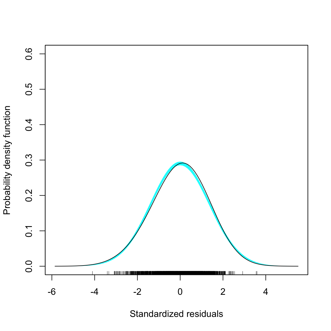
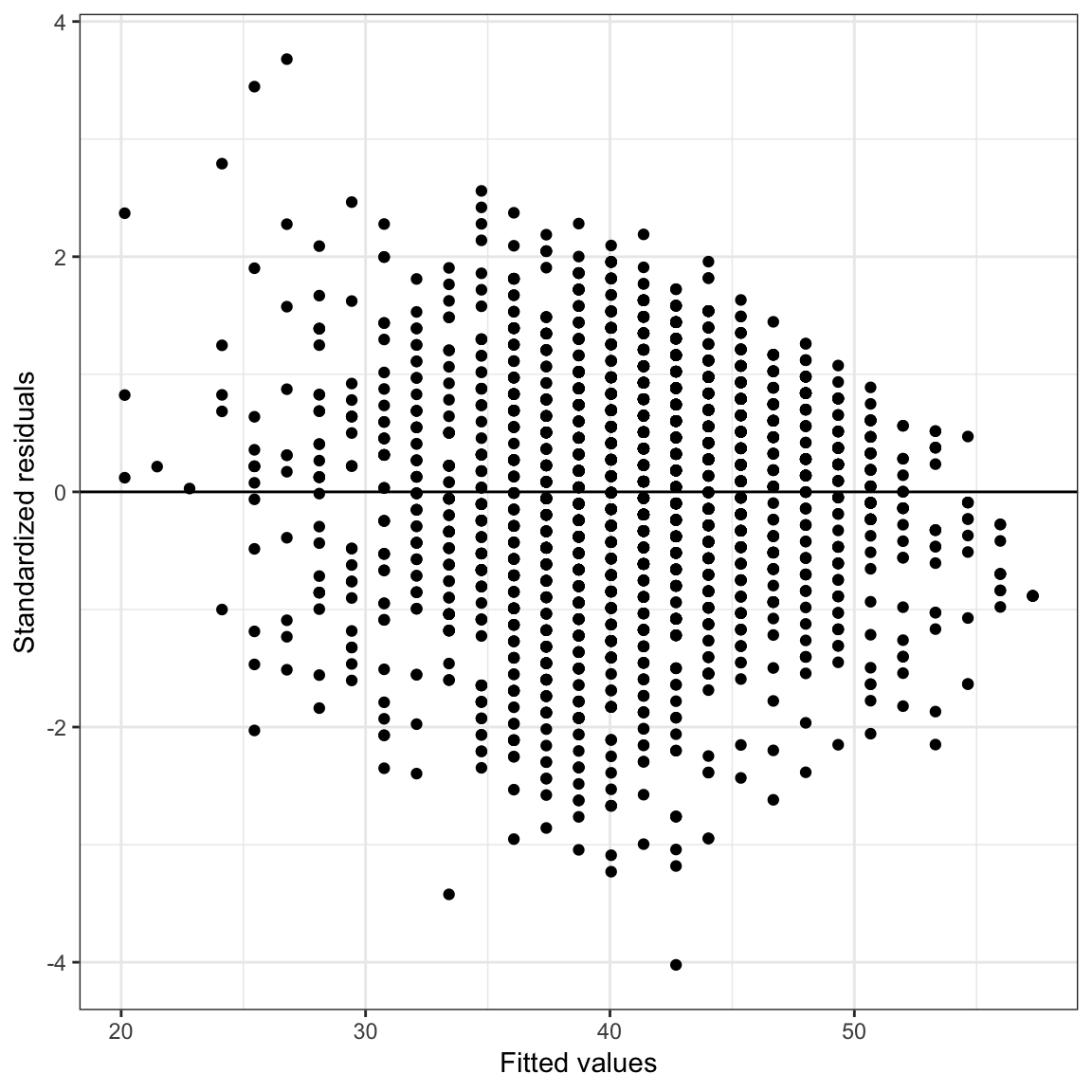
Figure 8.1: Density plot of the standardized residuals and scatterplot of the standardized residuals versus the fitted values from the fixed-effects regression model.
The assumption that the mean residual is 0 seems reasonably satisfied, however those of normality and homoscedasticity seem less feasible, especially given the large sample size. More importantly, the assumption of independence (which we don’t evaluate from the common residual plots) is probably not tenable. Students’ post-test language scores (and thus the residuals) are probably correlated within schools—this is a violation of independence which assumes that the correlation between student’s residuals is 0. If we have a variable that identifies classroom, we can actually examine this by plotting the residuals separately for each classroom.
In our case, we do have a variable that identifies classroom (school_id). We need to mutate this variable into the augmented dataset. This variable has 131 different levels, which means that we would be looking at 131 different residual plots. When we use facet_wrap() with that many levels each plot will be too small to see, so we will instead select a random sample of, say, 25 of the classrooms to evaluate.
# Make random sample reproducible
set.seed(100)

# Draw random sample of 25 schools without replacement
my_sample = sample(school_data$school_id, size = 25, replace = FALSE)

# Mutate on school ID and draw random sample
out = out %>%
  mutate(school_id = joined_data$school_id) %>%
  filter(school_id %in% my_sample)

### Show residuals by school
ggplot(data = out, aes(x = .fitted, y = .std.resid)) +
    geom_point() +
    geom_hline(yintercept = 0) +
    theme_bw() +
  xlab("Fitted values") +
  ylab("Studentized residuals") +
    facet_wrap(~school_id, nrow = 5)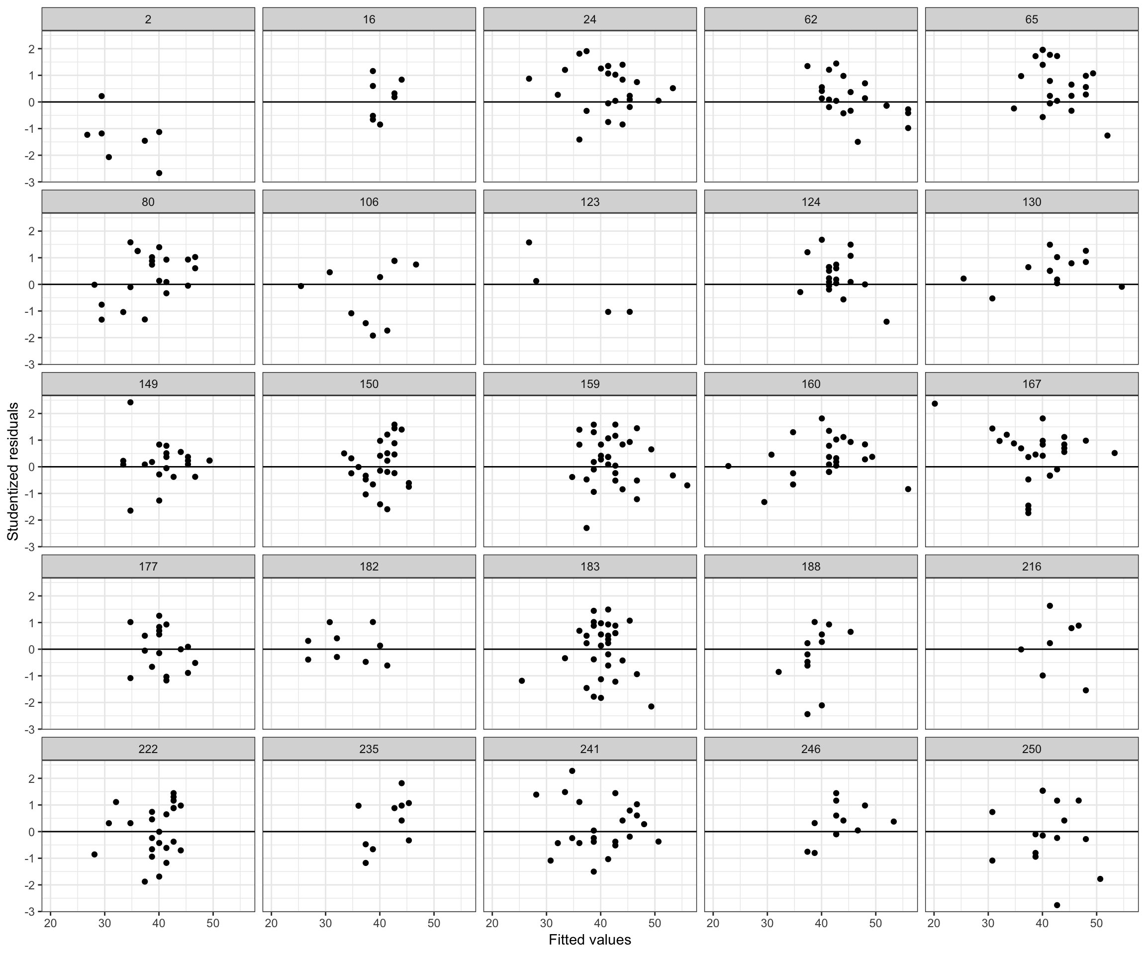
Figure 8.2: Scatterplots of the standardized residuals versus the fitted values from the fixed-effects regression model stratified by team.
The residuals for several of the schools show a systematic trends of being primarily positive or negative within schools. For example, the residuals for several schools (e.g., 47, 256 258) are primarily negative. This is a sign of non-independence of the residuals. If we hadn’t had the school ID variable we could have still made a logical argument about this non-independence via substantive knowledge. For example, students who attend a “high performing” will likely tend to have positive residuals (scores above average relative to the population), even after accounting for their verbal IQ scores.
To account for this within-school correlation we need to use a statistical model that accounts for the correlation among the residuals within schools. This is what mixed-effects models bring to the table. By correctly modeling the non-independence, we get more accurate standard errors and p-values.
Another benefit of using mixed-effects models is that we also get estimates of the variation accounted for at both the school- and student-levels. This disaggregating of the variation allows us to see which level is explaining more variation and to study predictors appropriate to explaining that variation. For example, suppose that you disaggregated the variation in language scores and found that:
- 96% of the variation in these scores was at the student-level, and
- 3% of the variation in these scores was at the classroom-level, and
- 1% of the variation in these scores was at the school-level.
By including school-level or classroom-level predictors in the model, you would only be “chipping away” at that 1% or 3%, respectively. You should focus your attention and resources on student-level predictors!
8.4 Conceptual Idea of Mixed-Effects Models
In this section we will outline the conceptual ideas behind mixed-effects models by linking the ideas behind these models to the conventional, fixed-effects regression model. It is important to realize that this is just conceptual in nature. Its purpose is only to help you understand the output you get from a mixed-effects model analysis.
To begin, we remind you of the fitted equation we obtained earlier from the fixed-effects regression:
\[ \hat{\mathrm{Language~Score}_i} = 34.19 + 2.04(\mathrm{Verbal~IQ}_i) \]
Mixed-effects regression actually fits a global model (like the one above) AND a school-specific model for each school. Conceptually, this is like fitting a regression model for each school separately. Below I show the results (for 5 of the schools) of fitting a different regression model to each school, but keep in mind that this is only to help you understand.
# Fit school models
school_models = joined_data %>%
  group_by(school_id) %>%
  do(mod = lm(language_post  ~ 1 + verbal_iq, data = .)) %>%
  tidy(mod) %>%
  head(., 10)

# View coefficients from fitted models
school_models
# A tibble: 10 x 6
# Groups: school_id [5]
school_id term estimate std.error statistic p.value
<dbl> <chr> <dbl> <dbl> <dbl> <dbl>
1 1 (Intercept) 39.8 1.58 25.1 3.16e-18
2 1 verbal_iq 2.24 0.541 4.14 3.98e- 4
3 2 (Intercept) 27.4 4.18 6.54 1.25e- 3
4 2 verbal_iq 1.28 1.22 1.06 3.40e- 1
5 10 (Intercept) 38.1 2.82 13.5 8.79e- 4
6 10 verbal_iq 5.76 1.43 4.02 2.76e- 2
7 12 (Intercept) 36.1 3.82 9.46 3.43e- 7
8 12 verbal_iq 2.18 1.42 1.54 1.48e- 1
9 15 (Intercept) 32.1 3.85 8.34 1.61e- 4
10 15 verbal_iq 3.71 1.71 2.16 7.36e- 2As an example, let’s focus on the fitted model for School 1.
\[ \hat{\mathrm{Language~Score}_i} = 39.79 + 2.24(\mathrm{Verbal~IQ}_i) \]
Comparing this school-specific model to the global model, we find that School 1’s intercept is higher than the intercept from the global model (by 5.65) and it’s slope is also higher than the slope from the global model (by 0.20). We can actually re-write the school-specific model using these ideas:
\[ \hat{\mathrm{Language~Score}_i} = \bigg[34.19 + 5.65\bigg] + \bigg[2.04 + 0.20\bigg](\mathrm{Verbal~IQ}_i) \]
In the language of mixed-effects modeling:
- The global intercept and slope are referred to as fixed-effects. (These are also sometimes referred to as between-groups effects.)
- The fixed-effect of intercept is \(34.19\); and
- The fixed effect of the slope is \(2.04\).
- The school-specific deviations from the fixed-effect values are referred to as random-effects. (These are also sometimes referred to as within-groups effects.)
- The random-effect of the intercept for School 1 is \(+5.65\); and
- The random-effect of the slope for School 1 is \(+0.20\).
Note, each school could potentially have a different random-effect for intercept and slope. For example, writing the team-specific fitted equation for School 2 in this manner,
\[ \begin{split} \hat{\mathrm{Language~Score}_i} &= 27.35 + 1.28(\mathrm{Verbal~IQ}_i)\\ &= \bigg[34.19 - 6.84\bigg] + \bigg[2.04 - 0.76\bigg](\mathrm{Verbal~IQ}_i).\\ \end{split} \]
In this model:
- The fixed-effects (global effects) are the same as they were for School 1.
- The fixed-effect of intercept is \(34.19\); and
- The fixed effect of the slope is \(2.04\).
- The random-effect of intercept for School 2 is \(-6.84\).
- The random-effect of slope for School 2 is \(-0.76\).
8.5 Fitting the Mixed-Effects Regression Model in Practice
In practice, we use the lmer() function from the lme4 library to fit mixed-effect regression models. This function will essentially do what we did in the previous section, but rather than independently fitting the team-specific models, it will fit all these models simultaneously and make use of the information in all the clusters (schools) to do this. This will result in better estimates for both the fixed- and random-effects.
The syntax looks similar to the syntax we use in lm() except now we split it into two parts. The first part of the syntax gives a model formula to specify the outcome and fixed-effects included in the model. This is identical to the syntax we used in the lm() function. In our example: language_post ~ 1 + verbal_iq indicating that we want to fit a model that includes fixed-effects for both the intercept and the effect of verbal IQ score.
We also have to declare that we want to fit a model for each school. To do this, we will include a random-effect for intercept. (We could also include a random-effect of verbal IQ, but to keep it simpler right now, we only include the RE of intercept.) The second part of the syntax declares this: (1 | school_id). This says fit school-specific models that vary in their intercepts. This is literally added to the fixed-effects formula using +. The complete syntax is:
# Fit mixed-effects regression model
lmer.1 = lmer(language_post ~ 1 + verbal_iq + (1 | school_id), data = joined_data)
To view the fixed-effects, we use the fixef() function.
fixef(lmer.1)(Intercept) verbal_iq
40.608 2.488 This gives the coefficients for the fixed-effects part of the model (i.e., the global model),
\[ \hat{\mathrm{Language~Score}_{ij}} = 40.61 + 2.49(\mathrm{Verbal~IQ}_{ij}) \]
Note that the notation now includes two subscripts. The i subscript still indicates the ith student, and the new j subscript indicates that the student was from the jth school. Since we accounted for school in the model (schools are allowed to have different intercepts) we need to now identify that in the equation. We interpret these coefficients from the fixed-effects equation exactly like lm() coefficients. Here,
- The predicted average post-test language score for students with a mean verbal IQ score (=0) is 40.61.
- Each one-point difference in verbal IQ score is associated with a 2.49-point difference in language scores, on average.
To view the school-specific random-effects, we use the ranef() function (only the first 5 rows are shown).
ranef(lmer.1)$school_id
(Intercept)
1 -0.37573940
2 -6.04469893
10 -3.66481710
12 -2.91463441
15 -5.74351132The random-effects indicate how the school-specific intercept differs from the overall average intercept. For example, the intercept for School 1 is approximately 0.38-points lower than the average intercept of 40.61 (the fixed-effect). This implies that, on average, students from School 1 with a mean verbal IQ score (=0) have an average post-test language score that is 0.38-points lower than their peers who also have a mean verbal IQ score.
From the estimated fixed- and random-effects, we can re-construct each school-specific fitted equation if we are so inclined. For example, to construct the school-specific fitted equation for School 1, we combine the estimated coefficients for the fixed-effects and the estimated random-effect for School 1:
\[ \begin{split} \hat{\mathrm{Language~Score}_{i}} &= \bigg[ 40.61 -0.376 \bigg]+ 2.49(\mathrm{Verbal~IQ}_{i}) \\[1ex] &= 40.2 + 2.49(\mathrm{Verbal~IQ}_{i}) \end{split} \]
In this notation, the j part of the subscript is dropped since j is now fixed to a specific school; \(j=1\).
8.6 Example 2: Life Satisfaction of NBA Players
As a second example, we will explore the question of whether NBA players’ success is related to life satisfaction. To do this, we will use two datasets, the nba-player-data.csv and nba-team-data.csv file (see the data codebook here). These data include player- and team-level attributes for \(n=300\) players and \(n=30\) teams, respectively. To begin, we will import both the player-level and team-level datasets and then join them together.
# Read in player-level data
nba_players = read_csv(file = "~/Documents/github/epsy-8252/data/nba-player-data.csv")

# Read in team-level data
nba_teams = read_csv(file = "~/Documents/github/epsy-8252/data/nba-team-data.csv")

# Join the datasets together
nba = nba_players %>%
  left_join(nba_teams, by = "team")

head(nba)
# A tibble: 6 x 6
player team success life_satisfacti… coach coach_experience
<chr> <chr> <dbl> <dbl> <chr> <dbl>
1 Daniel Ham… Atlanta … 0 12.1 Lloyd Pi… 0
2 Alex Poyth… Atlanta … 0 13.5 Lloyd Pi… 0
3 Jaylen Ada… Atlanta … 0 18.8 Lloyd Pi… 0
4 Miles Plum… Atlanta … 0 18 Lloyd Pi… 0
5 PJ Dozier Boston C… 0 12.2 Brad Ste… 2
6 Ed Davis Brooklyn… 0 16 Kenny At… 1We want to fit a model that regresses the life_satisfaction scores on the success values. In these data, however, we might expect that the life satisfaction of players is correlated within team. To account for that fact, we can include a random-effect of intercept in our regression model.
8.6.1 Fit the Mixed-Effects Model
Below we fit a mixed-effects regression model to predict variation in life satisfaction scores that includes success as a predictor. We also include a random-effect of intercept to account for the within-team correlation of life satisfaction scores. The statistical model is:
\[ \mathrm{Life~Satisfaction}_{ij} = \bigg[\beta_0 + b_{0j} \bigg] + \beta_1(\mathrm{Success}_{ij}) + \epsilon_{ij} \]
We fit the model using lmer() as:
# Fit model
lmer.1 = lmer(life_satisfaction ~ 1 + success + (1 | team), data = nba)
We can then extract the fixed-effects estimates using the fixef() function.
# Get fixed-effects
fixef(lmer.1)
(Intercept) success
11.575 1.666 We write the fitted fixed-effects model as:
\[ \hat{\mathrm{Life~Satisfaction}}_{ij} = 11.57 + 1.67(\mathrm{Success}_{ij}) \]
Again, we can interpret these fixed-effects estimates the same way we do any other regression coefficient.
- The predicted average life satisfaction for NBA players with a success score of 0 (free-throw percentage in the lowest 20%) is 11.57.
- Each one-unit difference in success (one-quantile difference) is associated with a 1.67-point difference in life satisfaction score, on average.
If we are interested in the fitted model for a SPECIFIC team, we can extract the random-effect of intercept for that team and add it to the fixed-effect intercept estimate. For example, the equation for the Minnesota Timberwolves is:
# Obtain random-effects
ranef(lmer.1)
$team
(Intercept)
Atlanta Hawks 2.7474
Boston Celtics 5.3594
Brooklyn Nets 4.1005
Charlotte Hornets 1.1515
Chicago Bulls -3.4811
Cleveland Cavaliers 0.9739
Dallas Mavericks -6.1708
Denver Nuggets 4.0877
Detroit Pistons -2.3659
Golden State Warriors -1.8955
Houston Rockets -2.3038
Indiana Pacers -1.4244
Los Angeles Clippers 5.5528
Los Angeles Lakers -5.0071
Memphis Grizzlies 0.6391
Miami Heat 0.6749
Milwaukee Bucks -5.8198
Minnesota Timberwolves 3.6616
New Orleans Pelicans -1.3426
New York Knicks -1.9479
Oklahoma City Thunder -1.5291
Orlando Magic -3.4961
Philadelphia 76ers 4.6167
Phoenix Suns -6.1341
Portland Trail Blazers 0.3600
Sacramento Kings -3.4140
San Antonio Spurs 0.1794
Toronto Raptors 3.8491
Utah Jazz 6.2954
Washington Wizards 2.0828\[ \begin{split} \hat{\mathrm{Life~Satisfaction}}_{i} &= \bigg[11.57 + 3.66 \bigg] + 1.67(\mathrm{Success}_{i}) \\[1ex] &= 15.23 + 1.67(\mathrm{Success}_{i}) \end{split} \]
For Timberwolves players,
- The predicted average life satisfaction for Timberwolves players with a success score of 0 (free-throw percentage in the lowest 20%) is 15.23. This is a score that is 3.66 points above average for all NBA players with a success score of 0.
- Each one-unit difference in success is associated with a 1.67-point difference in life satisfaction score for Timberwolves players, on average. This is the same rate-of-change as for NBA players in general.
As a comparison, we can also consider the equation for the Phoenix Suns:
\[ \begin{split} \hat{\mathrm{Life~Satisfaction}}_{i} &= \bigg[11.57 - 6.13 \bigg] + 1.67(\mathrm{Success}_{i}) \\[1ex] &= 5.44 + 1.67(\mathrm{Success}_{i}) \end{split} \]
- The predicted average life satisfaction for Suns players with a success score of 0 (free-throw percentage in the lowest 20%) is 5.44. This is a score that is 6.13 points below average for all NBA players with a success score of 0.
- Each one-unit difference in success is associated with a 1.67-point difference in life satisfaction score for Suns players, on average. This is the same rate-of-change as for NBA players in general.
Comparing these two team’s equations gives us some insight into why the effects are referred to as fixed-effects or random-effects.
\[ \begin{split} \mathbf{Timberwolves:~}\hat{\mathrm{Life~Satisfaction}}_{i} &= \bigg[11.57 + 3.66 \bigg] + 1.67(\mathrm{Success}_{i}) \\[1ex] \mathbf{Suns:~}\hat{\mathrm{Life~Satisfaction}}_{i} &= \bigg[11.57 - 6.13 \bigg] + 1.67(\mathrm{Success}_{i}) \\[1ex] \end{split} \]
In the two equations, the fixed-effects of intercept (11.57) and success (1.67) are represented in both equations; they are fixed. On the other hand, the random-effect is different for each team. Since we included a random-effect of intercept in out model, this means that the intercept value for each team equation will be different.