Log Transformations: Some Final Thoughts
There are four general curvilinear, monotonic functions (shown below).
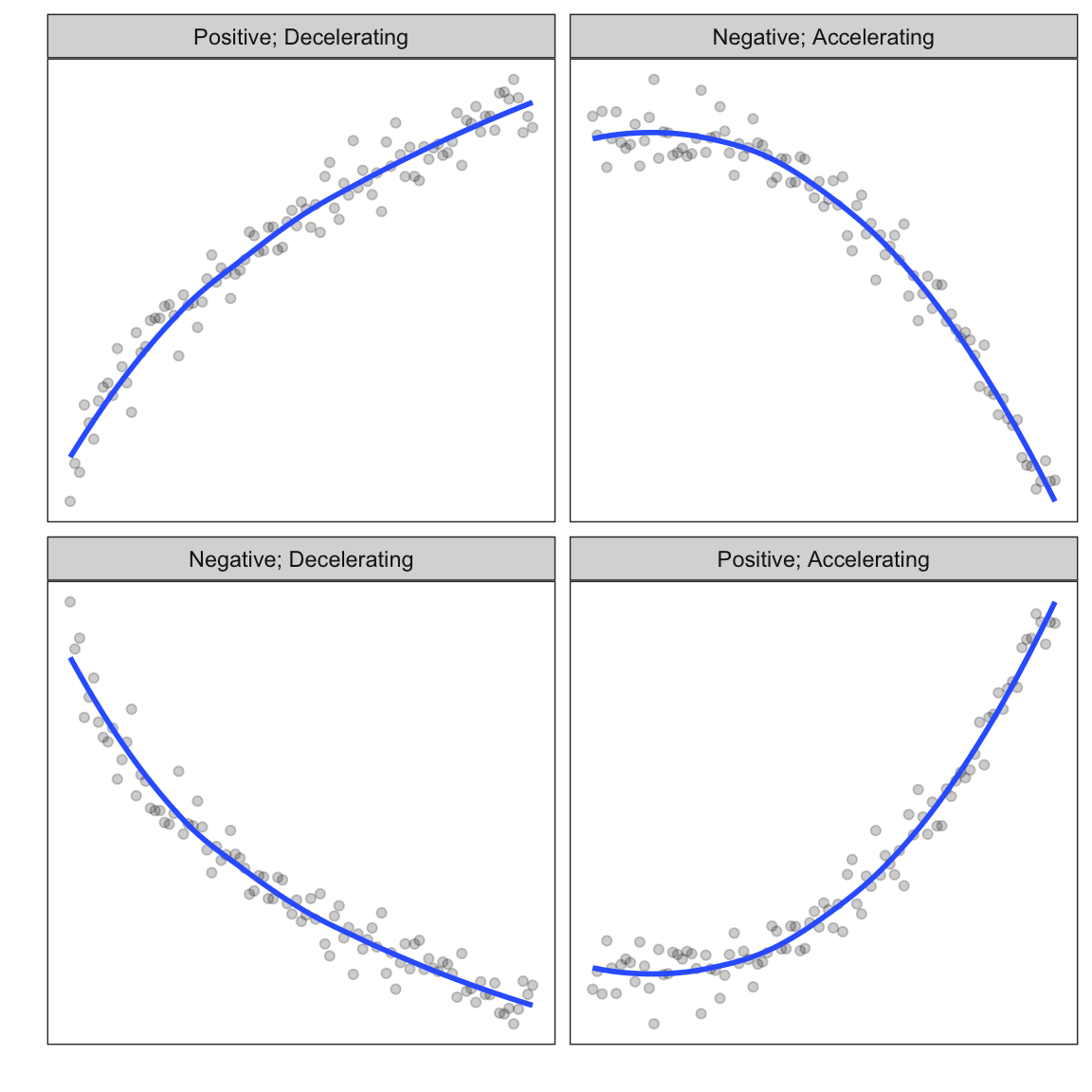
Figure 3.8: Four general monotonic, curvilinear shapes.
In the previous two units you learned how to transform the data to “linearize” two of the four monotonic functions:
- For positive, decelerating functions we log-transformed X; and
- For positive, accelerating functions we log-transformed Y.
To better understand how we can use transformations to straighten-out relationships, we will examine a set of transformations known as power transformations.
Power Transformations
Consider a set of powers, \(p\) that can be used in the exponent of a variable \(X\) (the variable is irrelevant; it could also be \(Y\)) so that a transformation of the variable \(X\) is:
\[ \mathrm{Transformed~Variable} = X^p \]
Consider the following values for \(p\):
\[ p = \{-3,-2,-1,0,1,2,3\} \]
These all represent particular transformations of \(X\). Note that when \(p=1\), the variable \(X\) is left untransformed (\(X^1 = X\)). Consider the following transformations:
\[ \begin{split} &X^3 \\ &X^2 \\ &X^1 \qquad \mathrm{Untransformed} \end{split} \]
These are shown in the figure below.
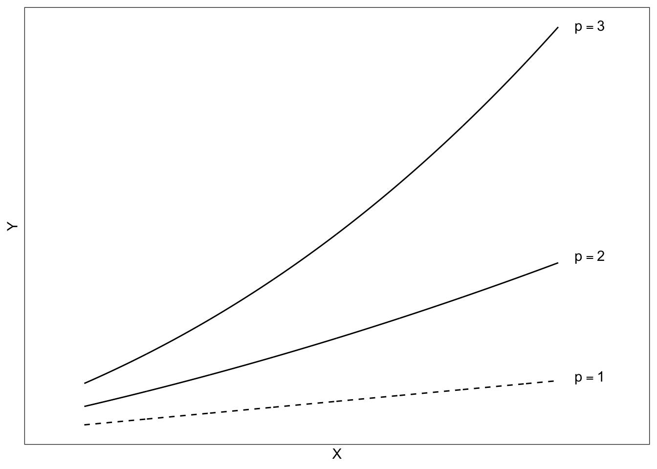
Power transformations that are bigger than 1 (\(p>1\)) show positive acceleration. Powers larger than one are referred to as upward transformations as they increase the power (move it up) from one.
Now consider these transformations:
\[ \begin{split} &X^{-1} \\ &X^{-2} \\ &X^{-3} \end{split} \]
These are shown in the figure below.
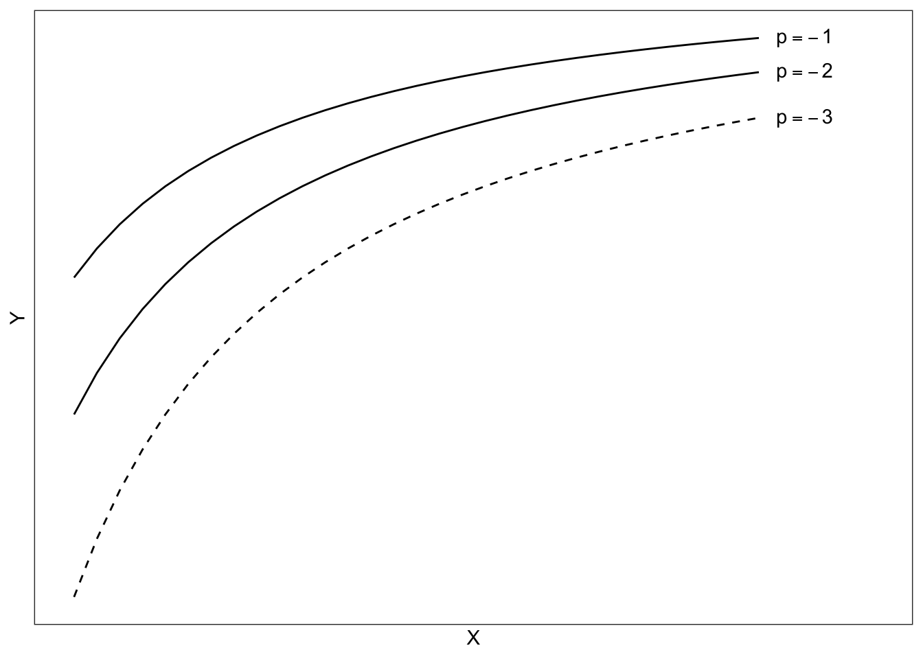
For power transformations that are smaller than 1 (\(p<1\)), the function shows positive deceleration. Powers that are smaller than one are referred to as downward transformations as they decrease the power (move it down) from one.
Ladder of Transformations
If we order the different values of \(p\), they form what statisticians call a “ladder of re-expression” or “ladder of transformations”.
\[ \begin{split} & ~~~~~\vdots \\ &Y^3,X^3 &\qquad \mathrm{Upward~Transformation}\\ &Y^2,X^2 &\qquad \mathrm{Upward~Transformation}\\ &Y^1,X^1 &\qquad \mathrm{Untransformed} \\ &Y^{\frac{1}{2}},X^{\frac{1}{2}} &\qquad \mathrm{Downward~Transformation}\\ &Y^0,X^0 \equiv \ln(X) &\qquad \mathrm{Downward~Transformation}\\ &Y^{-1},X^{-1} &\qquad \mathrm{Downward~Transformation}\\ &Y^{-2},X^{-2} &\qquad \mathrm{Downward~Transformation}\\ &Y^{-3},X^{-3} &\qquad \mathrm{Downward~Transformation} \\ & ~~~~~\vdots \end{split} \]
Rule of the Bulge
To determine how we need to transform data, we can rely on Mosteller and Tukey’s ‘Rule of the Bulge’. This rule, depicted visually below, has us “move on the ladder in the direction in which the bulge points”.
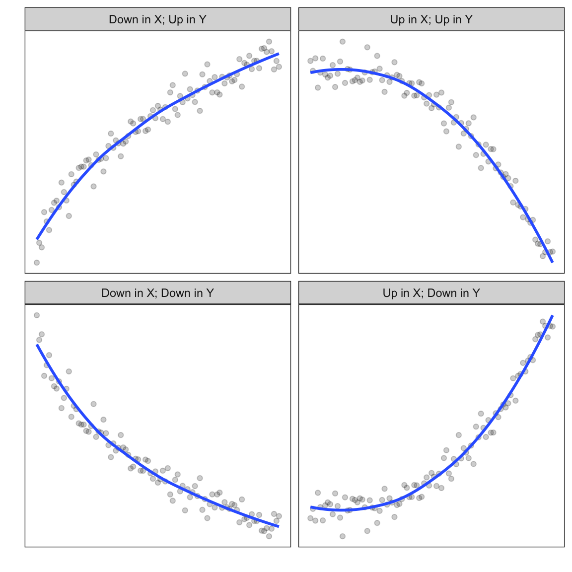
Figure 3.9: Four general monotonic, curvilinear shapes. The Rule of the Bulge helps us identify how to transform the data to linearize any of these four shapes.
For example, below we re-visit the mn-schools.csv data and again look at the relationship between median SAT score and six-year graduation rate.
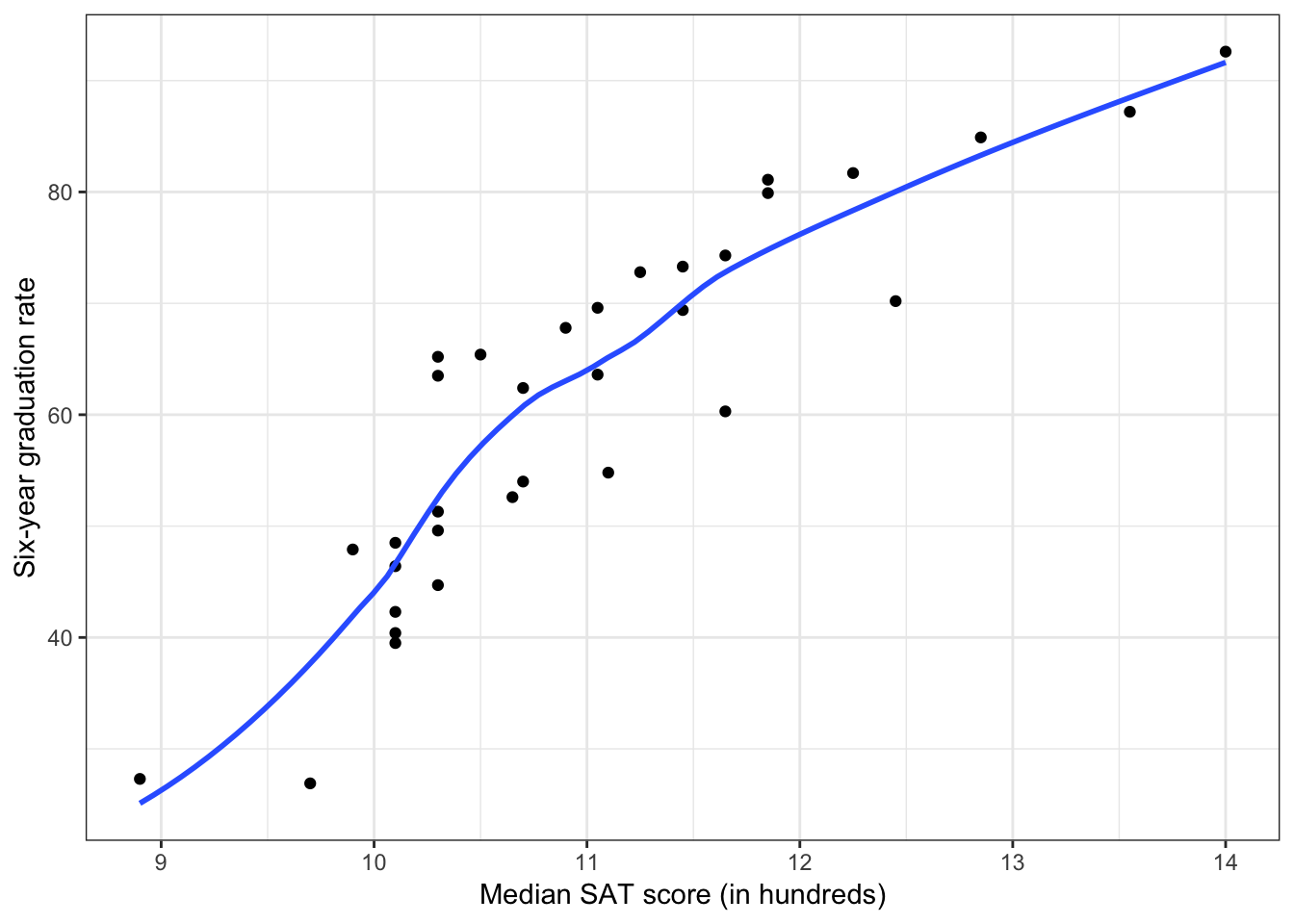
Figure 3.10: Scatterplot of the relationship between median SAT score and six-year graduation rate. The loess smoother is also displayed.
This positive, decelerating relationship is similar to the one in the upper-lefthand quadrant of the ‘Rule of the Bulge’. To linearize this we can either:
- Transform \(X\) using a DOWNWARD transformation; or
- Transform \(Y\) using an UPWARD transformation.
In the Unit 2 notes, we linearized this by taking the natural logarithm of SAT; a downward transformation of \(X\). What about the relationship between movie age and budget we looked at in Unit 3?
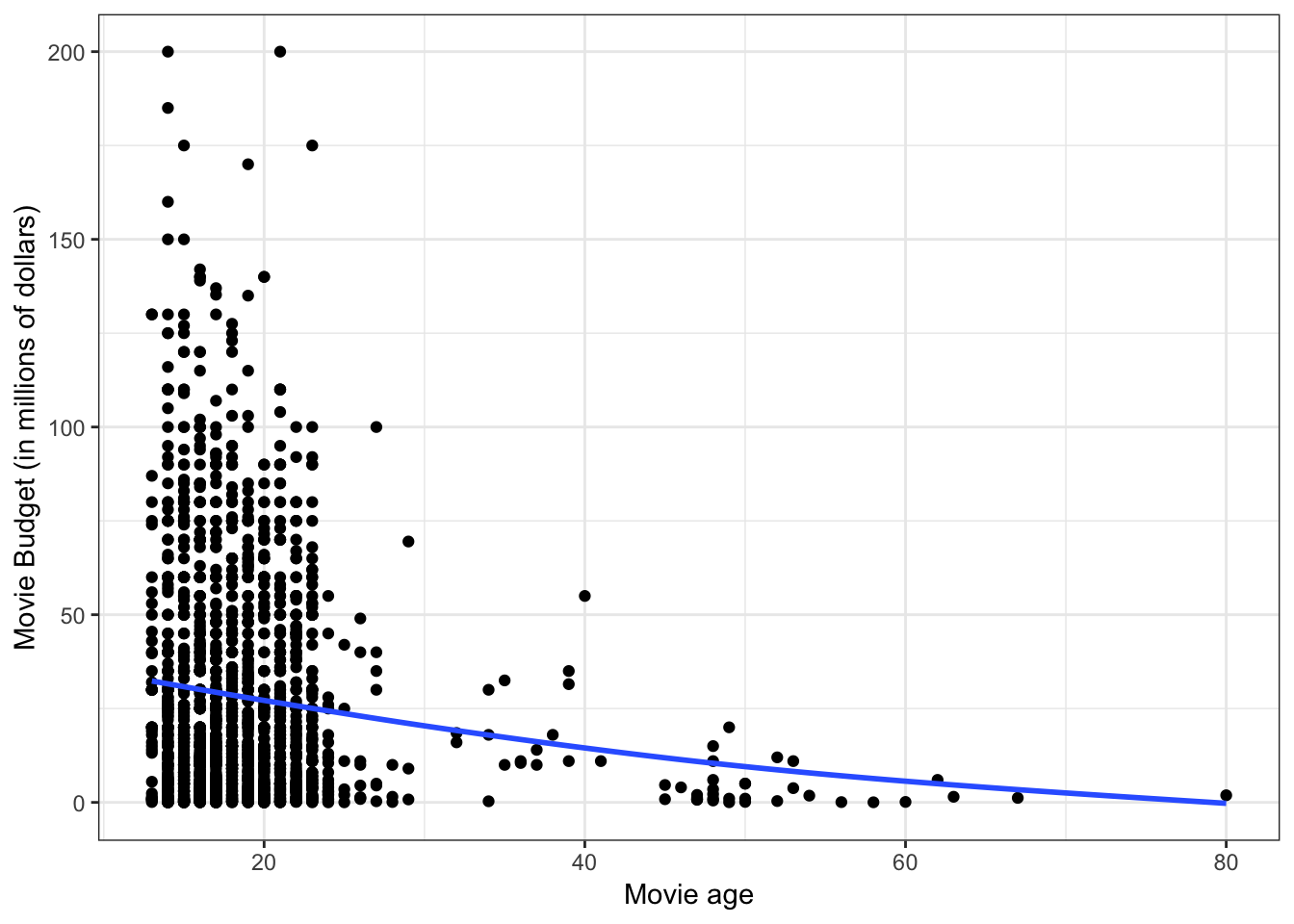
Figure 3.11: Scatterplot between age and budget. The loess smoother is also displayed.
This negative, decelerating relationship is similar to the one in the lower-lefthand quadrant of the ‘Rule of the Bulge’. To linearize this we can either:
- Transform \(X\) using a DOWNWARD transformation; or
- Transform \(Y\) using an DOWNWARD transformation.
In the Unit 3 notes, we linearized this by taking the natural logarithm of budget; a downward transformation of \(Y\). By transforming \(Y\) instead of \(X\), we also fixed a problem of heterogeneity of variance; a problem in the residuals (which is related to \(Y\)).