Unit 3: Nonlinearity: Log-Transforming the Outcome
In this set of notes, you will learn about log-transforming the outcome variable in a regression model to account for nonlinearity and heterogeneity of variance.
Preparation
Before class you will need to read the following:
- Osborne, Jason (2002). Notes on the use of data transformations. Practical Assessment, Research & Evaluation, 8(6).
3.1 Dataset and Research Question
The data we will use in this set of notes, movies.csv (see the data codebook here), includes attributes for \(n=1,806\) movies.
# Load libraries
library(broom)
library(dplyr)
library(ggplot2)
library(readr)
library(sm)
library(tidyr)

# Import data
movies = read_csv(file = "~/Documents/github/epsy-8252/data/movies.csv")
head(movies)
# A tibble: 6 x 4
title budget age mpaa
<chr> <dbl> <dbl> <chr>
1 'Til There Was You 23 21 PG-13
2 10 Things I Hate About You 16 19 PG-13
3 100 Mile Rule 1.1 16 R
4 13 Going On 30 37 14 PG-13
5 13th Warrior, The 85 19 R
6 15 Minutes 42 17 R Using these data, we will examine the relationship between age of a movie and budget.
3.2 Examine Relationship between Age and Budget
To being the analysis, we will examine the scatterplot between age and budget of our sample data.
ggplot(data = movies, aes(x = age, y = budget)) +
  geom_point() +
  geom_smooth(se = FALSE) +
  theme_bw() +
  xlab("Movie age") +
  ylab("Movie Budget (in millions of dollars)")
Figure 3.1: Scatterplot between age and budget. The loess smoother is also displayed.
The scatterplot suggests two potential problems with fitting a linear model to the data:
- The relationship is slightly curvilinear.
- The variation in budget for more recent movies is much greater than the variation in budget for older movies (heteroskedasticity).
We can see this much more clearly in the scatterplot of residuals versus fitted values from a fitted linear model.
# Fit model
lm.1 = lm(budget ~ 1 + age, data = movies)

# Obtain residuals and fitted values
out_1 = augment(lm.1)

# Density plot of the residuals
sm.density(out_1$.std.resid, model = "normal", xlab = "Standardized residuals")

# Residuals versus fitted values
ggplot(data = out_1, aes(x = .fitted, y = .std.resid)) +
  geom_point() +
  geom_hline(yintercept = 0) +
  geom_smooth() +
  theme_bw() +
  xlab("Fitted values") +
  ylab("Standardized residuals")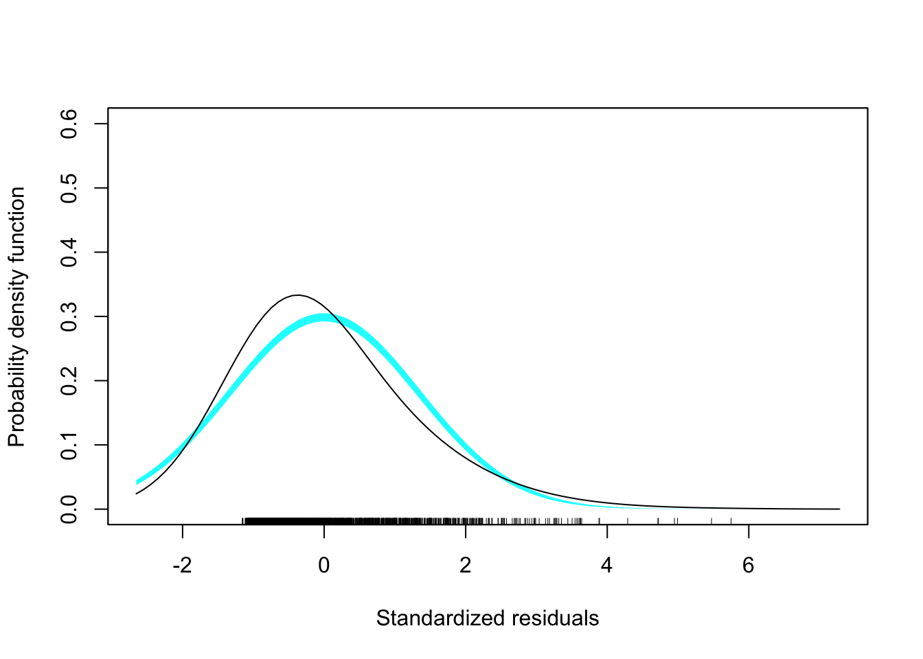
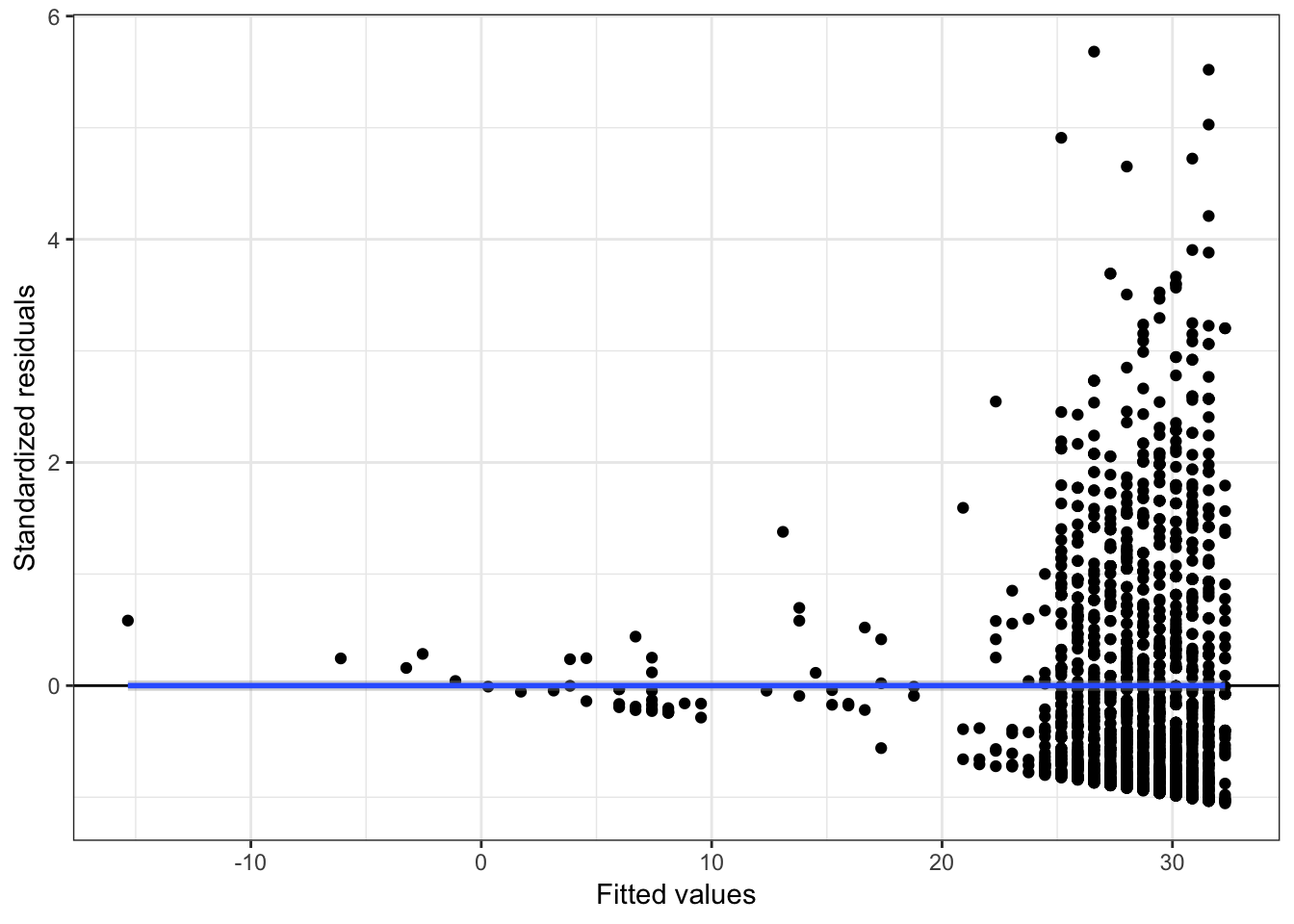
Figure 3.2: Residual plots from regressing budget on age.
These plots suggest violations of the normality assumption (the marginal distribution of the residuals is right-skewed) and of the assumption of homoskedasticity. Because of the large sample size, violation the linearity assumption is more difficult to see in this plot.
3.3 Transform the Outcome Using the Natural Logarithm (Base-e)
To alleviate problems of non-normality when the conditional distributions are right-skewed (or have high-end outliers) OR to alleviate heteroskedasticity, we can mathematically transform the outcome using a logarithm. Any base can be used for the logarithm, but we will transform the outcome using the natural logarithm because of the interpretive value.
First, we will create the log-transformed variable as a new column in the data, and then we will use the log-transformed budget (rather than raw budget) in any analyses.
# Create log-transformed budget
movies = movies %>%
  mutate(
    Lbudget = log(budget)
    )

# Examine data
head(movies)
# A tibble: 6 x 5
title budget age mpaa Lbudget
<chr> <dbl> <dbl> <chr> <dbl>
1 'Til There Was You 23 21 PG-13 3.14
2 10 Things I Hate About You 16 19 PG-13 2.77
3 100 Mile Rule 1.1 16 R 0.0953
4 13 Going On 30 37 14 PG-13 3.61
5 13th Warrior, The 85 19 R 4.44
6 15 Minutes 42 17 R 3.74 Recall that the logarithm is the inverse function of an exponent. As an example, consider the budget and log-transformed budget for ’Til There Was You.
\[ \begin{split} \ln(\textrm{Budget}) &= 3.135 \\ \ln(23.0) &= 3.135 \\ \end{split} \]
Or,
\[ e^{3.135} = 23.0 \]
Remember, the logarithm answers the mathematical question:
\(e\) to what power is equal to 23.0?
3.4 Re-analyze using the Log-Transformed Budget
Now we will re-examine the scatterplot using the log-transformed outcome to see how this transformation affects the relationship.
# Scatterplot
ggplot(data = movies, aes(x = age, y = Lbudget)) +
  geom_point() +
  geom_smooth(se = FALSE) +
  theme_bw() +
  xlab("Movie age") +
  ylab("ln(Movie Budget)")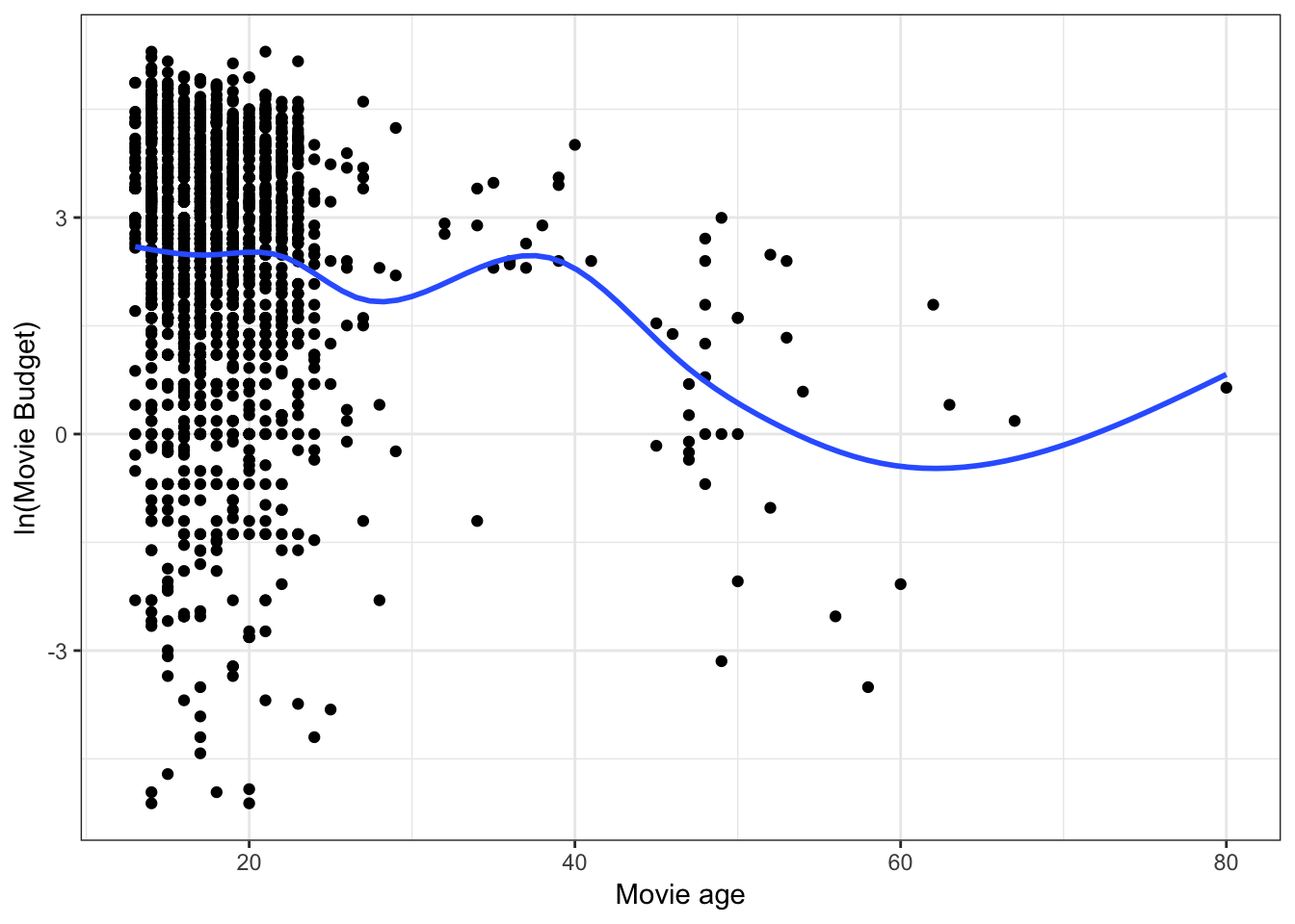
Figure 3.3: Scatterplot between age and log-transformed budget. The loess smoother is also displayed.
Log-transforming the outcome has drastically affected the scale for the outcome. Has this helped us better meet the assumptions? Again, we should examine the residual plots.
# Fit model
lm.2 = lm(Lbudget ~ 1 + age, data = movies)

# Obtain residuals and fitted values
out_2 = augment(lm.2)

# Density plot of the residuals
sm.density(out_2$.std.resid, model = "normal", xlab = "Standardized residuals")

# Residuals versus fitted values
ggplot(data = out_2, aes(x = .fitted, y = .std.resid)) +
  geom_point() +
  geom_hline(yintercept = 0) +
  geom_smooth() +
  theme_bw() +
  xlab("Fitted values") +
  ylab("Standardized residuals")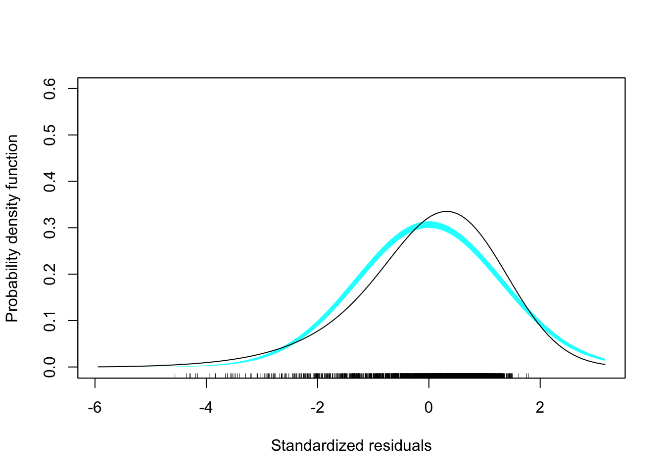
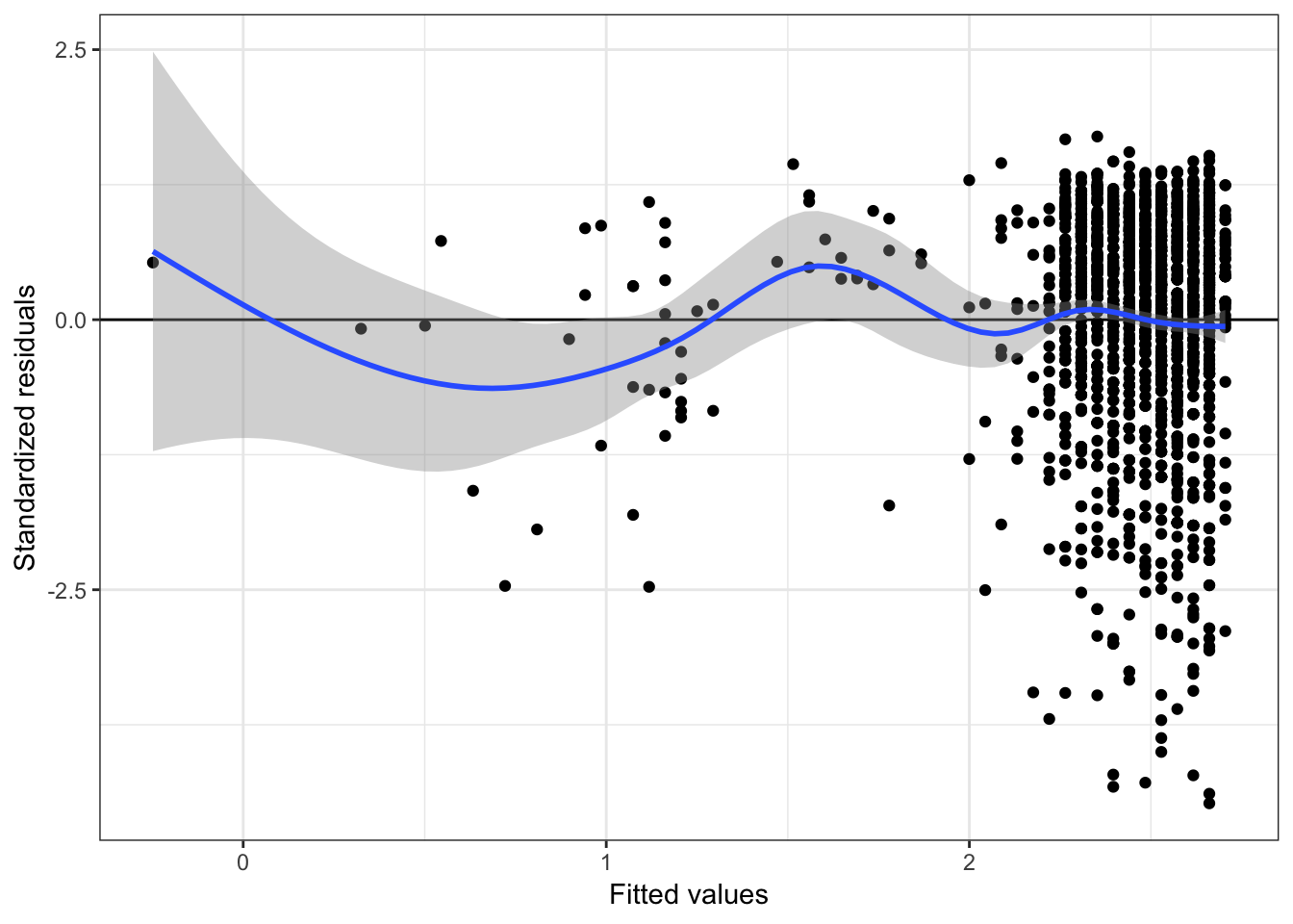
Figure 3.4: Residual plots from regressing the natural logarithm of budget on age.
These plots still suggest violations of the normality assumption (the marginal distribution of the residuals is now left-skewed). The assumption of homoskedasticity also seems still violated, although much less. Most importantly, however, is the assumption of linearity now seems satisfied.
3.5 Interpreting the Regression Output
Let’s examine the output from the model in which we regressed the log-transformed budget on age.
# Model-level output
glance(lm.2)
# A tibble: 1 x 11
r.squared adj.r.squared sigma statistic p.value df logLik AIC BIC
<dbl> <dbl> <dbl> <dbl> <dbl> <int> <dbl> <dbl> <dbl>
1 0.0213 0.0208 1.74 39.3 4.60e-10 2 -3560. 7125. 7142.
# … with 2 more variables: deviance <dbl>, df.residual <int>The model-level summary information suggests that differences in movies’ ages explains 2.1% of the variation in budget. (Remember, explaining variation in log-budget is the same as explaining variation in budget). Although this is a small amount of variation, it is statistically significant, \(F(1,1804)=39.27\), \(p<0.001\).
# Coefficient-level output
tidy(lm.2)
# A tibble: 2 x 5
term estimate std.error statistic p.value
<chr> <dbl> <dbl> <dbl> <dbl>
1 (Intercept) 3.28 0.139 23.6 1.69e-107
2 age -0.0441 0.00703 -6.27 4.60e- 10From the coefficient-level output the fitted equation is:
\[ \ln\left(\hat{\mathrm{Budget}_i}\right) = 3.28 - 0.04(\mathrm{Age}_i) \]
With log-transformations, there are two possible interpretations we can offer. The first is to interpret the coefficients using the log-transformed values. These we interpret in the exact same way we do any other regression coefficients (except we use log-outcome instead of outcome):
- The intercept, \(\hat{\beta_0} = 3.28\), is the average predicted log-budget for movies made in 2019 (Age = 0).
- The slope, \(\hat{\beta_1} = -0.04\), indicates that each one-year difference in age is associated with a log-budget that differ by \(-0.04\), on average.
3.5.1 Back-Transforming: A More Useful Interpretation
A second, probably more useful, interpretation is to back-transform log-budget to budget. To think about how to do this, we first consider a more general expression of the fitted linear model:
\[ \ln\left(\hat{Y}_i\right) = \hat\beta_0 + \hat\beta_1(X_{i}) \]
The left-hand side of the equation is in the log-transformed metric, which drives our interpretations. If we want to instead, interpret using the raw metric of \(Y\), we need to back-transform from \(\ln(Y)\) to \(Y\). To back-transform, we use the inverse function, which is to exponentiate using the base of the logarithm, in our case, base-\(e\).
\[ e^{\ln(Y_i)} = Y_i \]
If we exponentiate the left-hand side of the equation, to maintain the equality, we also need to exponentiate the right-hand side of the equation.
\[ e^{\ln(Y_i)} = e^{\hat\beta_0 + \hat\beta_1(X_{i})} \]
Then we use rules of exponents to simplify this.
\[ Y_i = e^{\hat\beta_0} \times e^{\hat\beta_1(X_{i})} \]
For our example, when we exponentiate both sides of the fitted equation:
\[ \hat{\mathrm{Budget}_i} = e^{3.28} \times e^{-0.04(\mathrm{Age}_i)} \]
3.5.2 Substituting in Values for Age to Interpret Effects
To interpret the effects (which are now interpreted using budget—not log-budget) we can substitute in the different values for age and solve. For example when Age = 0:
\[ \begin{split} \hat{\mathrm{Budget}_i} &= e^{3.28} \times e^{-0.04(0)}\\ &= 26.58 \times 1 \\ &= 26.58 \end{split} \]
The predicted budget for a movie made in 2019 is 26.58 million dollars. How about a movie that was made in 2018 (a one-year difference)?
\[ \begin{split} \hat{\mathrm{Budget}_i} &= e^{3.28} \times e^{-0.04(1)}\\ &= 26.58 \times 0.96 \\ &= 25.54 \end{split} \]
The predicted budget for a movie made in 2019 is 25.54 million dollars. This is 0.96 TIMES the budget of a movie made in 2018.
Rather than using the language of TIMES difference you could also use the language of fold difference. In this case the slope coefficient would be interpreted as,
Each one-year difference in age is associated with a 0.95-fold difference in budget, on average.
Simply put, when we back-transform from interpretations of log-\(Y\) to \(Y\) the interpretations are multiplicatively related to the intercept rather than additive. We can obtain these multiplicative values (and the back-transformed intercept) by using the exp() function to exponentiate the coefficients from the fitted model, which we obtain using the coef() function.
exp(coef(lm.2))(Intercept) age
26.5261 0.9569 3.5.3 Approximate Interpretation of the Slope
Remember that by using the natural logarithm we can interpret the effects as percent change. Rather than saying that a movie made in 2018 is predicted to have a budget that is 0.96 TIMES that of a movie made in 2019, we can directly interpret the slope as the percent change. Thus \(\hat{\beta_1}=-0.04\) can be interpreted as:
Each one-year difference in age is associated with a four percent decrease in budget, on average.
If you want the specific mathematical change in budget, find \(1 - e^{\hat{\beta_1}}\).
1 - exp(-0.04)[1] 0.03921If you use the language of percent decrease/increase, be very careful. Percent change and percentage change are sometimes interpreted differently! It is generally more clear to use the X-fold difference language.
3.6 Plotting the Fitted Model
As always, we can plot the fitted model to aid in interpretation. To do this we will create a sequence of ages, predict the log-budget using the fitted model, and then back-transform the log-budgets to raw budget.
# Set up data
plot_data = crossing(
    age = seq(from = 13, to = 80, by = 1)
    ) %>%
  mutate(
    # Predict
    yhat = predict(lm.2, newdata = .)
  )

# Examine data
head(plot_data)
# A tibble: 6 x 2
age yhat
<dbl> <dbl>
1 13 2.71
2 14 2.66
3 15 2.62
4 16 2.57
5 17 2.53
6 18 2.48# Back-transform the log-budgets
plot_data = plot_data %>%
mutate(
budget = exp(yhat)
)
# Examine data
head(plot_data)# A tibble: 6 x 3
age yhat budget
<dbl> <dbl> <dbl>
1 13 2.71 15.0
2 14 2.66 14.3
3 15 2.62 13.7
4 16 2.57 13.1
5 17 2.53 12.5
6 18 2.48 12.0# Plot
ggplot(data = plot_data, aes(x = age, y = budget)) +
geom_line() +
theme_bw() +
xlab("Age") +
ylab("Predicted budget (in millions of U.S. dollars)")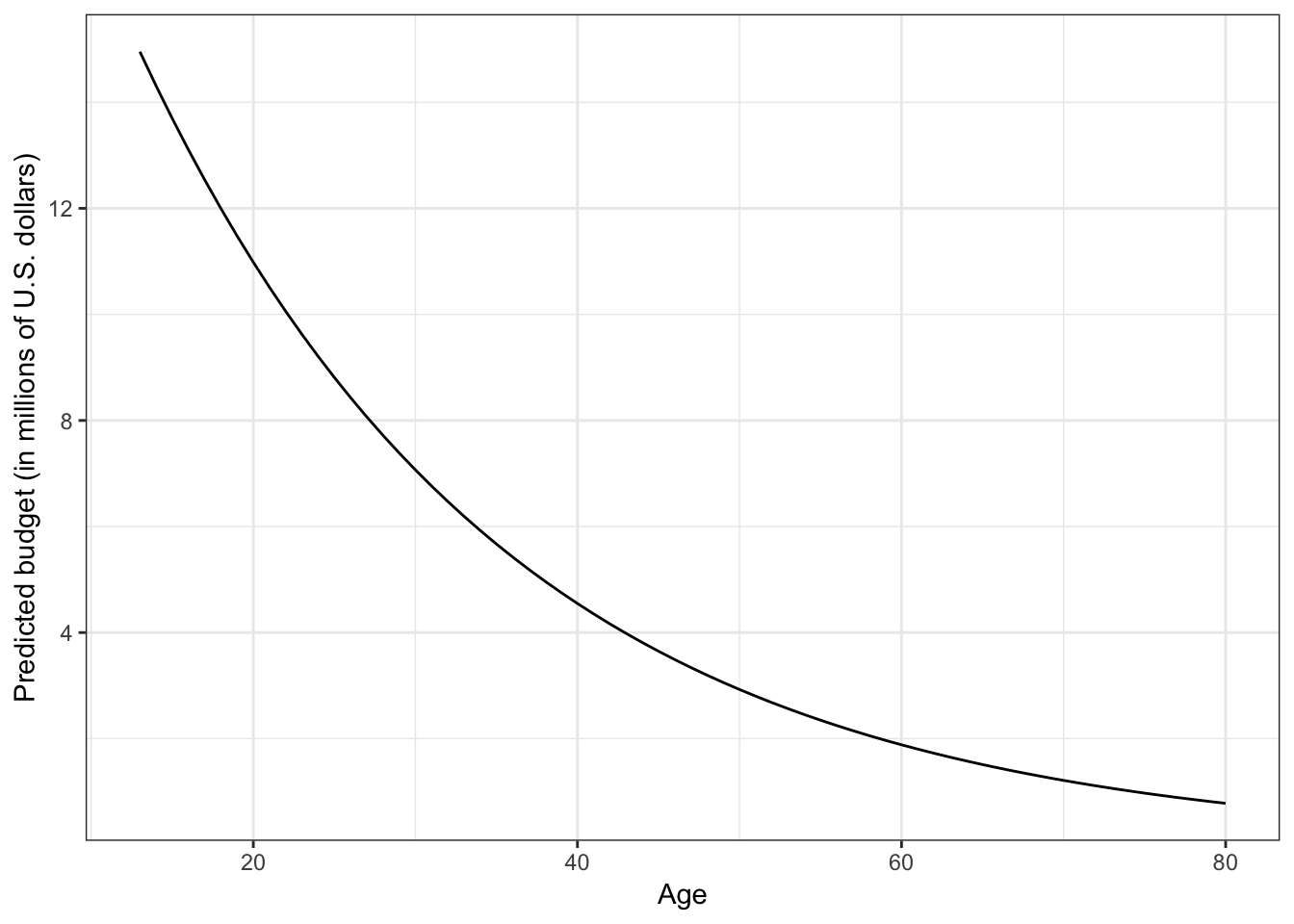
Figure 3.5: Plot of the predicted movie budget as a function of its age. The non-linearity in the plot indicates that there is a diminishing negative effect of age on budget.
Based on this plot, we see the non-linear, negative effect of age on budget. In other words, older movies tend to have a smaller budget, on average, but this decrease is not constant. This pattern of non-linear decline is referred to as exponential decay.
Although this function has a different look than the function we saw in the previous unit (it is negative rather than positive), it is also a monotonic function (no change in direction).
3.7 Relationship between MPAA Rating and Budget
We also may want to control for differences in MPAA rating. Before we fit the multiple regression model, however, we will first explore whether MPAA rating is a useful covariate by seeing whether there are differences in budget between PG, PG-13m and R rated movies. Since we log-transformed budget (the outcome) in the previous analysis we will need to use the log-transformed outcome in this exploration as well.
# Plot the observed data
ggplot(data = movies, aes(x = mpaa, y = Lbudget)) +
  geom_jitter(alpha = 0.2) +
  stat_summary(fun.y = 'mean', geom = "point", size = 4, color = "darkred") +
    theme_bw() +
    xlab("MPAA rating") +
    ylab("ln(Movie Budget)")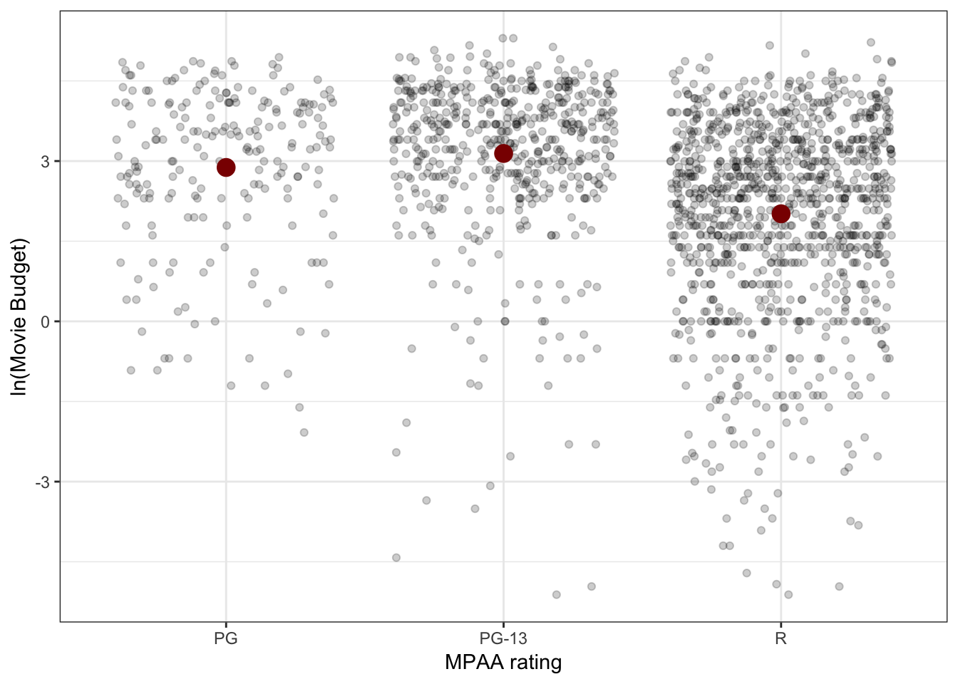
Figure 3.6: Jittered scatterplot of log-budget versus MPAA rating.
# Compute summary statistics
movies %>%
  group_by(mpaa) %>%
  summarize(
    M = mean(Lbudget),
    SD = sd(Lbudget)
    )
# A tibble: 3 x 3
mpaa M SD
<chr> <dbl> <dbl>
1 PG 2.88 1.53
2 PG-13 3.14 1.51
3 R 2.01 1.78The scatterplot and summary statistics indicate there are sample differences in the mean log-budgets for the three MPAA ratings. The variation in log-budgets seems roughly the same for the three ratings.
3.7.1 Regression Model
Let’s regress log-transformed budget on MPAA rating and examine the output from the model. To do so, we will need to first create three dummy variables for the different ratings.
# Create dummy variables
movies = movies %>%
  mutate(
    pg   = if_else(mpaa == "PG", 1, 0),
    pg13 = if_else(mpaa == "PG-13", 1, 0),
    r    = if_else(mpaa == "R", 1, 0)
  )

# Fit the model (pg is reference group)
lm.3 = lm(Lbudget ~ 1 + pg13 + r, data = movies)

# Model-level output
glance(lm.3)
# A tibble: 1 x 11
r.squared adj.r.squared sigma statistic p.value df logLik AIC BIC
<dbl> <dbl> <dbl> <dbl> <dbl> <int> <dbl> <dbl> <dbl>
1 0.0892 0.0882 1.68 88.3 2.66e-37 3 -3495. 6997. 7019.
# … with 2 more variables: deviance <dbl>, df.residual <int>The model-level summary information suggests that differences in MPAA rating explains 8.9% of the variation in budget. (Remember, explaining variation in log-budget is the same as explaining variation in budget). Although this is a small amount of variation, it is statistically significant, \(F(2,1803)=88.28\), \(p<0.001\).
# Coefficient-level output
tidy(lm.3)
# A tibble: 3 x 5
term estimate std.error statistic p.value
<chr> <dbl> <dbl> <dbl> <dbl>
1 (Intercept) 2.88 0.115 25.0 9.98e-119
2 pg13 0.262 0.136 1.92 5.45e- 2
3 r -0.867 0.126 -6.88 8.49e- 12From the coefficient-level output we see that the fitted equation is:
\[ \ln\left(\hat{\mathrm{Budget}_i}\right) = 2.88 + 0.26(\mathrm{PG\mbox{-}13}_i) - 0.87(\mathrm{R}_i) \]
With log-transformations, there are two possible interpretations we can offer. The first is to interpret the coefficients using the log-transformed values. These we interpret in the exact same way we do any other regression coefficients (except we use log-outcome instead of outcome):
- The intercept, \(\hat{\beta_0} = 2.88\), is the average predicted log-budget for PG rated movies.
- The slope associated with PG-13, \(\hat{\beta_1} = 0.26\), indicates that PG-13 rated movies have a log-budget that is 0.26 higher than PG rated movies, on average.
- The slope associated with R, \(\hat{\beta_2} = -0.87\), indicates that R rated movies have a log-budget that is 0.87 lower than PG rated movies, on average.
We can also interpret these by back-transforming to raw budget. To do that we exponentiate the coefficients.
exp(coef(lm.3))(Intercept) pg13 r
17.8134 1.2998 0.4201 - PG rated movies have a budget of 17.81 million dollars, on average.
- PG-13 rated movies have a budget that is 1.30 TIMES the estimated budget for PG rated movies, on average.
- R rated movies have a budget that is 0.42 TIMES the estimated budget for PG rated movies, on average.
3.7.2 Mathematical Explanation
Remember, if we want to interpret using the raw metric of \(Y\), we need to back-transform from \(\ln(Y)\) to \(Y\). To back-transform, we use the inverse function, which is to exponentiate using the base of the logarithm, in our case, base-\(e\). For our example, when we exponentiate both sides of the fitted equation:
\[ \begin{split} e^{\ln\left(\hat{\mathrm{Budget}_i}\right)} &= e^{2.88 + 0.26(\mathrm{PG\mbox{-}13}_i) - 0.87(\mathrm{R}_i)} \\ \hat{\mathrm{Budget}_i} &= e^{2.88} \times e^{0.26(\mathrm{PG\mbox{-}13}_i)} \times e^{-0.87(\mathrm{R}_i)} \end{split} \]
To interpret the effects (which are now interpreted using budget—not log-budget) we can substitute in the different dummy variable patterns and solve.
\[ \begin{split} \textbf{PG Movie:}~~ \hat{\mathrm{Budget}_i} &= e^{2.88} \times e^{0.26(0)} \times e^{-0.87(0)}\\ &= 17.81 \times 1 \times 1 \\ &= 17.81 \end{split} \]
\[ \begin{split} \textbf{PG-13 Movie:}~~ \hat{\mathrm{Budget}_i} &= e^{2.88} \times e^{0.26(1)} \times e^{-0.87(0)}\\ &= 17.81 \times 1.30 \times 1 \\ &= 23.15 \end{split} \]
\[ \begin{split} \textbf{R Movie:}~~ \hat{\mathrm{Budget}_i} &= e^{2.88} \times e^{0.26(0)} \times e^{-0.87(1)}\\ &= 17.81 \times 1 \times 0.42 \\ &= 7.48 \end{split} \]
3.7.3 Approximate Interpretations
Unfortunately, the approximate interpretations of the slopes by directly interpreting the coefficients using the language of percent change are not completely trustworthy. If we did interpret them, the interpretations for the two slopes would be:
- PG-13 rated movies have budget that is 26.2 percent higher than PG rated movies, on average.
- R rated movies have budget that is 87 percent lower than PG rated movies, on average.
This interpretation is roughly true for the PG-13 effect, but not for the R effect. This approximate interpretation starts to become untrustworthy when the slope value is higher than about 0.20 or so.
3.8 Multiple Regression: Main Effects Model
Now we can fit a model that includes our focal predictor of age and our covariate of MPAA rating.
# Fit model (PG is reference group)
lm.4 = lm(Lbudget ~ 1 + age + pg13 + r, data = movies)

# Model-level output
glance(lm.4)
# A tibble: 1 x 11
r.squared adj.r.squared sigma statistic p.value df logLik AIC BIC
<dbl> <dbl> <dbl> <dbl> <dbl> <int> <dbl> <dbl> <dbl>
1 0.109 0.108 1.66 73.8 4.82e-45 4 -3474. 6959. 6986.
# … with 2 more variables: deviance <dbl>, df.residual <int>The model-level summary information suggests that differences in age and MPAA rating of a movie explains 11.0% of the variation in budget. (Remember, explaining variation in log-budget is the same as explaining variation in budget); \(F(3,1802)=73.84\), \(p<0.001\).
# Coefficient-level output
tidy(lm.4)
# A tibble: 4 x 5
term estimate std.error statistic p.value
<chr> <dbl> <dbl> <dbl> <dbl>
1 (Intercept) 3.73 0.175 21.3 3.76e-90
2 age -0.0431 0.00673 -6.41 1.89e-10
3 pg13 0.208 0.135 1.54 1.23e- 1
4 r -0.904 0.125 -7.24 6.79e-13The coefficient-level output suggest that there is still a statistically significant effect of age on budget, after controlling for differences in MPAA rating; \(t(1802)=-6.41\), \(p<.001\).
To determine if there is an effect of MPAA rating, after accounting for differences in age, at least one of the effects of MPAA rating need to be statistically significant. Here we see that the coefficient associated with rated R movies is statistically significant.
Remember that when we have more than two categories (more than one dummy variable) there can be many ways for the effect to play out, and not all of these are represented in the model we fitted. One way we can simultaneously examine ALL the ways this effect can play out is to use a nested \(F\)-test.
3.8.1 Nested F-Test
If we want to examine if there is a controlled effect of MPAA rating (controlling for age), we want to see whether by including MPAA rating in a model THAT ALREADY INCLUDES age we explain additional variation in the outcome. To do this we can compare a model that only includes the effect of age to a model that includes both the effects of age and MPAA rating. If the latter model explains a statistically significant amount of additional variation we can say that there is an effect of MPAA rating after controlling for differences in age.
In statistical hypothesis testing we are examining the following null hypothesis:
\[ H_0: \rho^2_{\mathrm{Age},\mathrm{MPAA~rating}} - \rho^2_{\mathrm{Age}} = 0 \]
If we fail to reject this hypothesis, then the two models explain the SAME amount of variation and we should adopt the simpler model; MPAA rating does not explain additional variation in budget. If we reject this hypothesis, MPAA rating does explain additional variation in budget, above and beyond age; and we should adopt the model that includes both effects.
To test this hypothesis we fit both models and then give both models to the anova() function.
# Fit models
lm.2 = lm(Lbudget ~ 1 + age,            data = movies)
lm.4 = lm(Lbudget ~ 1 + age + pg13 + r, data = movies)

# Nested F-test
anova(lm.2, lm.4)
Analysis of Variance Table
Model 1: Lbudget ~ 1 + age
Model 2: Lbudget ~ 1 + age + pg13 + r
Res.Df RSS Df Sum of Sq F Pr(>F)
1 1804 5448
2 1802 4957 2 491 89.2 <2e-16 ***
---
Signif. codes: 0 '***' 0.001 '**' 0.01 '*' 0.05 '.' 0.1 ' ' 1The test suggests that there is a statistically significant effect of MPAA rating even after accounting for differences in age; \(F(2, 1802)=89.21\), \(p<.001\).
3.8.2 Coefficient-Level Interpretation
To interpret the coefficients, we will again exponentiate the fitted coefficients so we can interpret them using the raw-metric of budget.
exp(coef(lm.4))(Intercept) age pg13 r
41.7120 0.9578 1.2318 0.4051 - The model estimated budget for a PG movie (reference group) that was made in 2019 (age = 0) is 41.71 million dollars.
- Each one-year difference in age is associated with a 0.96-fold difference (4.3% decrease) in budget, on average, controlling for differences in MPAA rating.
- PG-13 rated movies have a budget that is 1.23 times that for PG movies, on average, controlling for differences in age.
- R rated movies have a budget that is 0.41 times that for PG movies, on average, controlling for differences in age.
3.8.3 Plot of the Fitted Model
To plot the fitted model that includes a categorical predictor with more than two levels, it is best to re-fit the lm() using the categorical variable.
# Re-fit the model
lm.5 = lm(Lbudget ~ 1 + age + mpaa, data = movies)

# Model-level output
glance(lm.5)
# A tibble: 1 x 11
r.squared adj.r.squared sigma statistic p.value df logLik AIC BIC
<dbl> <dbl> <dbl> <dbl> <dbl> <int> <dbl> <dbl> <dbl>
1 0.109 0.108 1.66 73.8 4.82e-45 4 -3474. 6959. 6986.
# … with 2 more variables: deviance <dbl>, df.residual <int># Coefficient-level output
tidy(lm.5)# A tibble: 4 x 5
term estimate std.error statistic p.value
<chr> <dbl> <dbl> <dbl> <dbl>
1 (Intercept) 3.73 0.175 21.3 3.76e-90
2 age -0.0431 0.00673 -6.41 1.89e-10
3 mpaaPG-13 0.208 0.135 1.54 1.23e- 1
4 mpaaR -0.904 0.125 -7.24 6.79e-13Note this is the exact same model we fitted using the dummy variables, but R will choose the reference group for us (alphabetically). We can now set up our plotting data, predict, back-transform the outcome, and plot.
# Set up data
plot_data = crossing(
    age = seq(from = 13, to = 80, by = 1),
    mpaa = c("PG", "PG-13", "R")
    ) %>%
  mutate(
    yhat = predict(lm.5, newdata = .),
    budget = exp(yhat)
  )

# Examine data
head(plot_data)
# A tibble: 6 x 4
age mpaa yhat budget
<dbl> <chr> <dbl> <dbl>
1 13 PG 3.17 23.8
2 13 PG-13 3.38 29.3
3 13 R 2.27 9.65
4 14 PG 3.13 22.8
5 14 PG-13 3.34 28.1
6 14 R 2.22 9.24# Plot
ggplot(data = plot_data, aes(x = age, y = budget, color = mpaa, linetype = mpaa)) +
geom_line() +
theme_bw() +
xlab("Age") +
ylab("Predicted budget (in millions of U.S. dollars)") +
ggsci::scale_color_d3(name = "MPAA rating") +
scale_linetype_manual(name = "MPAA rating", values = 1:3)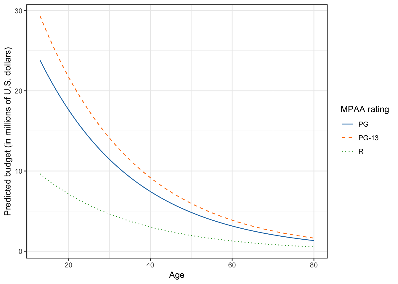
Figure 3.7: Plot of the predicted movie budget as a function of its age and MPAA rating. The non-linearity in the plot indicates that there is a diminishing negative effect of age on budget.
The plot displays the negative, nonlinear effect of age on budget for all three types of movies (main effect of age). It also shows that PG-13 rated movies have a higher predicted budget than PG and R rated movies, and that PG rated movies have a higher predicted budget than R rated movies at EVERY age. This is the main effect of MPAA rating.
Notice that in the plot, the three lines are not parallel. This is a mathematical artifact of back-transforming log-budget to raw budget. It does not indicate that an interaction model was fitted. How non-parallel the lines are depends on the size of the coefficients associated with the MPAA effects (in this example). This is why, especially with transformed data, it is essential to plot the model to make sure you are understanding the interpretations from your coefficients.
3.9 Multiple Regression: Interaction Model
To study whether there is an interaction effect between MPAA rating and age, we will fit the interaction model and compare it to the main-effects model using the nested \(F\)-test.
# Fit the models
lm.5 = lm(Lbudget ~ 1 + age + mpaa,            data = movies)
lm.6 = lm(Lbudget ~ 1 + age + mpaa + age:mpaa, data = movies)

# Nested F-test
anova(lm.5, lm.6)
Analysis of Variance Table
Model 1: Lbudget ~ 1 + age + mpaa
Model 2: Lbudget ~ 1 + age + mpaa + age:mpaa
Res.Df RSS Df Sum of Sq F Pr(>F)
1 1802 4957
2 1800 4949 2 7.76 1.41 0.24The test suggests that we should adopt the main-effects model. The interaction-effect was not statistically significant; \(F(2,1800)=1.41\), \(p=.244\).
If the model that included the interaction effect was adopted, it would suggest that: (1) the effect of age on budget depends on MPAA rating, or (2) the effect of MPAA rating on budget depends on age of the movie. To further interpret these effects, you should plot the results of the fitted interaction model.