
Chapter 16 Basis Vectors and Matrices
In this chapter, you will learn about basis vectors and basis matrices and how they are used to define the dimensionality of a coordinate space. You will also learn how to transition to different coordinate systems by changing the basis vectors.
16.1 An Example
In the chapter Vectors, we learned that a vector could be represented in a coordinate system where each element in the vector corresponds to a distance along one of the reference axes defining the coordinate system. For example, the vector:
\[ \mathbf{a} = \begin{bmatrix} -3 \\ 4 \end{bmatrix} \]
has a distance of \(-3\) on the first reference axis (R1) and a distance of 4 on the second reference axis (R2). This vector and the reference axes are shown in Figure 16.1. The reference axes (R1 and R2) define a two-dimensional coordinate space.
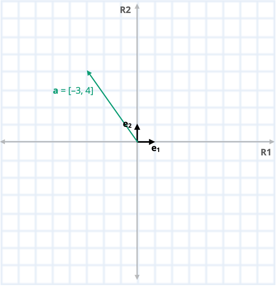
Figure 16.1: Plot showing vector a (in teal) in the R1–R2 dimensional space.
The two-dimensional coordinate system in our example, the Cartesian coordinate system, is defined by two orthogonal vectors called the basis vectors because they form the basis for the two-dimensional space. (These are shown in black in Figure 16.1.) More specifically, the dimensions of a system are determined by the number of independent vectors within that system. For example, in a three-dimensional coordinate space there are three independent vectors (e.g., that form the x, y, and z axes).
The span of the basis vectors create what we think of as the axes for that system. In our example, we have two basis vectors whose spans create R1 and R2. There are many possible sets of basis vectors whose spans would create R1 and R2, but the standard basis is the set of elementary vectors, in two-dimensional space:
\[ \mathbf{e}_1 = \begin{bmatrix} 1 \\ 0 \end{bmatrix} \qquad\mathbf{e}_2 = \begin{bmatrix} 0 \\ 1 \end{bmatrix} \]
Here the two basis vectors are orthogonal and have unit length. We refer to vectors that have these properties as orthonormal.
We can represent any vector in the space as a linear combination of a set of scalars and the basis vectors. For example consider the vector:
\[ \mathbf{a} = \begin{bmatrix} -3 \\ 4 \end{bmatrix} \]
We can also express a as:
\[ \begin{split} \mathbf{a} &= -3 \begin{bmatrix} 1 \\ 0 \end{bmatrix} + 4 \begin{bmatrix} 0 \\ 1 \end{bmatrix} \\[2em] &= -3\mathbf{e}_1 + 4\mathbf{e}_2 \end{split} \]
In general a vector a is can be expressed relative to the basis vectors as:
\[ \mathbf{a} = a_1(\mathbf{e}_1) + a_2(\mathbf{e}_2) + a_3(\mathbf{e}_3) + \dots + a_n(\mathbf{e}_n) \]
where \(\mathbf{e}_i\) is the ith orthonormal basis vector.
16.2 Changing Basis Vectors
There is nothing sacred about the Cartesian coordinate system. We could also define the two-dimensional space using a different set of orthonormal basis vectors. For example consider the basis vectors:
\[ \mathbf{b}_1 = \begin{bmatrix} \frac{\sqrt{2}}{2} \\ -\frac{\sqrt{2}}{2} \end{bmatrix} \qquad\mathbf{b}_2 = \begin{bmatrix} \frac{\sqrt{2}}{2} \\ \frac{\sqrt{2}}{2} \end{bmatrix} \]
These basis vectors still are orthonormal—they are orthogonal and their length is one. However, they are not elementary vectors. Not all orthonormal vectors are elementary vectors. R1 and R2 are still defined as the spans of these vectors, but now the vector a (which had the coordinates \(-3, 4\) in the system defined by the standard basis) has a different set of coordinates in the new basis. We can see this in 16.2.
Figure 16.2: Plot showing vector a (in teal) in the R1–R2 dimensional space with basis vectors b1 and b2.
The coordinates in the new basis for a is:
\[ \mathbf{a}=\begin{bmatrix} -4.95 \\ 0.707 \end{bmatrix} \]
To find the coordinates of a vector a under a non-standard basis, we can express a using the new basis vectors as:
\[ \begin{split} \mathbf{a} &= a_1(\mathbf{b}_1) + a_2(\mathbf{b}_2) \\[2ex] &= a_1\begin{bmatrix} \frac{\sqrt{2}}{2} \\ -\frac{\sqrt{2}}{2} \end{bmatrix} + a_2\begin{bmatrix} \frac{\sqrt{2}}{2} \\ \frac{\sqrt{2}}{2} \end{bmatrix} \end{split} \]
Then, since a has coordinates (\(-3,4\)) in the standard system, we can re-write this as:
\[ \begin{split} \begin{bmatrix}-3 \\ 4 \end{bmatrix} &= a_1\begin{bmatrix} \frac{\sqrt{2}}{2} \\ -\frac{\sqrt{2}}{2} \end{bmatrix} + a_2\begin{bmatrix} \frac{\sqrt{2}}{2} \\ \frac{\sqrt{2}}{2} \end{bmatrix} \\[2ex] &= \begin{bmatrix} \frac{\sqrt{2}}{2} & \frac{\sqrt{2}}{2} \\ -\frac{\sqrt{2}}{2} & \frac{\sqrt{2}}{2} \end{bmatrix}\begin{bmatrix}a_1 \\ a_2\end{bmatrix} \end{split} \] Now we need to solve for the values of \(a_1\) and \(a_2\). Note the basis vectors form the columns of the basis matrix, and we can solve for the values of \(a_1\) and \(a_2\) by pre-multiplying both sides by the inverse of the basis matrix.
# Create basis matrix
B = matrix(
  data = c(sqrt(2)/2, -sqrt(2)/2, sqrt(2)/2, sqrt(2)/2),
  nrow = 2
  )

# Create a
a = matrix(
  data = c(-3, 4),
  nrow = 2
  )

# Solve for the values of the new coordinates
solve(B) %*% a
[,1]
[1,] -4.9497475
[2,] 0.707106816.2.1 Non-Orthonormal Basis
There is no specification that the basis vectors need to be orthogonal, or have length of one. For example consider the basis vectors:
\[ \mathbf{b}_1 = \begin{bmatrix} \frac{\sqrt{2}}{2} \\ \frac{\sqrt{2}}{2} \end{bmatrix} \qquad\mathbf{b}_2 = \begin{bmatrix} 1.8 \\ 0.2 \end{bmatrix} \]
Here the basis vectors are no longer orthogonal. We refer to non-orthogonal vectors as oblique. The second basis vector also has a length which is no longer one. In this basis, the vector a (which had the coordinates \(-3, 4\) in the system defined by the standard basis) has yet a different set of coordinates; seen in 16.3.
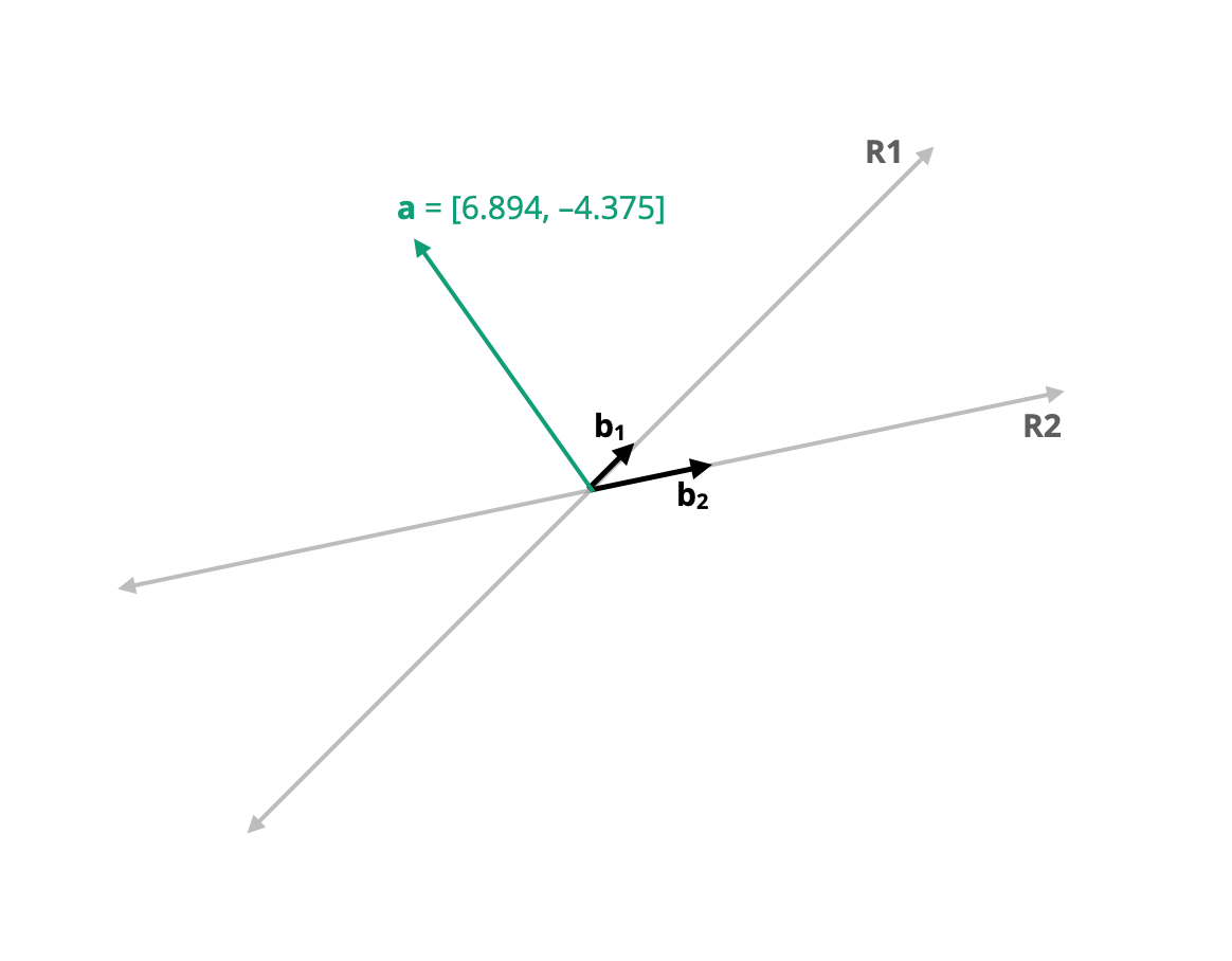
Figure 16.3: Plot showing vector a (in teal) in the R1–R2 dimensional space with the oblique basis vectors b1 and b2.
To find the coordinates in the oblique basis, we solve
\[ \begin{bmatrix}-3 \\ 4 \end{bmatrix} = \begin{bmatrix} \frac{\sqrt{2}}{2} & 1.8 \\ \frac{\sqrt{2}}{2} & 0.2 \end{bmatrix} \begin{bmatrix}a_1 \\ a_2\end{bmatrix} \]
As long as the basis matrix is conformable, we can solve this for \(a_1\) and \(a_2\).
# Create basis matrix
B = matrix(
  data = c(sqrt(2)/2, sqrt(2)/2, 1.8, 0.2),
  nrow = 2
  )

# Create a
a = matrix(
  data = c(-3, 4),
  nrow = 2
  )

# Solve for the values of the new coordinates
solve(B) %*% a
[,1]
[1,] 6.894291
[2,] -4.375000The coordinates for a in the new basis is:
\[ \mathbf{a} = \begin{bmatrix}6.894 \\ -4.375\end{bmatrix} \]
16.3 Converting Non-Standard Coordinates to the Standard Basis
We can, given a set of coordinates for a vector in a non-standard basis system, transform this to the coordinates of a vector in the standrd basis system. For example, consider the vector a, which has coordinates defined in the basis given by B:
\[ \mathbf{a} = \begin{bmatrix}3 \\ 2\end{bmatrix} \qquad \mathbf{B} = \begin{bmatrix} \frac{\sqrt{2}}{2} & 1.8 \\ \frac{\sqrt{2}}{2} & 0.2 \end{bmatrix} \]
What are the coordinates of this vector in the standard basis system? 16.3 shows this graphically.
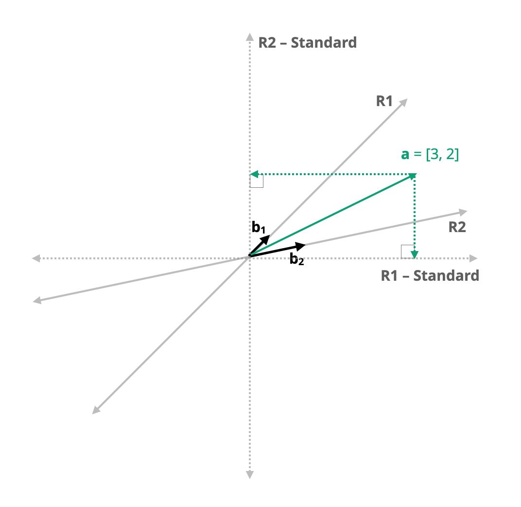
Figure 16.4: Plot showing vector a (in teal) in the R1–R2 non-standard basis defined by b1 and b2. The coordinates in the standard basis are found by determining the projection onto the span of the standard basis vectors (i.e., the R1 and R2 axes in the standard basis).
To find the coordinates of a in the standard basis system, we need to find the projections onto the spans of the standard basis vectors. To do this, we can use the same equation we have been using to convert coordinates to a non-standard basis. Recall, this equation is:
\[ \mathbf{a}_{[\mathrm{S}]} = \mathbf{B}_{[\mathrm{NS}]}\mathbf{a}_{[\mathrm{NS}]} \]
where \(\mathbf{a}_{[\mathrm{S}]}\) is the vector a in the standard basis, \(\mathbf{a}_{[\mathrm{NS}]}\) is the vector a in the non-standard basis, and \(\mathbf{B}_{[\mathrm{NS}]}\) is the basis matrix defining the non-standard system. To determine the coordinates for a in the standard system, we simply postmultiply the non-standard basis matrix by the vector a in the non-standard system.
# Create basis matrix
B = matrix(
  data = c(sqrt(2)/2, sqrt(2)/2, 1.8, 0.2),
  nrow = 2
  )

# Create a (non-standard)
a = matrix(
  data = c(3, 2),
  nrow = 2
  )

# Find a (standard)
B %*% a
[,1]
[1,] 5.72132
[2,] 2.52132The coordinates for a in the standard basis sytem is:
\[ \mathbf{a} = \begin{bmatrix}5.721 \\ 2.521\end{bmatrix} \]
16.4 Final Thoughts
Although we have been working in two dimensions so it is easier to show these ideas visually, basis vectors and matrices can, of course, be expanded to define coordinate systems in higher dimensions. For example, to define the standard three-dimensional space, we use the following basis vectors:
\[ \mathbf{e}_1 = \begin{bmatrix} 1 \\ 0 \\ 0 \end{bmatrix} \qquad\mathbf{e}_2 = \begin{bmatrix} 0 \\ 1 \\ 0 \end{bmatrix} \qquad\mathbf{e}_3 = \begin{bmatrix} 0 \\ 0 \\ 1 \end{bmatrix} \]
which can be expressed as the basis matrix B:
\[ \mathbf{B} = \begin{bmatrix} 1 & 0 & 0\\ 0 & 1 & 0 \\ 0 & 0 & 1 \end{bmatrix} \]
In general, to define an n-dimensional space, we need n basis vectors of dimension \(n \times 1\), which create an \(n \times n\) basis matrix. This implies that the basis matrix will be square.
When we have a linear combinations that take on the form:
\[ \underset{n \times 1}{\mathbf{y}} = \underset{n \times n}{\mathbf{B}} ~\underset{n \times 1}{\mathbf{x}} \] where y and x are vectors and B is a square matrix, then y is the projection of the vector x (which is defined using the basis matrix B) onto the set of standard basis vectors.