Chapter 7 Matrices

A matrix is a rectangular array of elements arranged in rows and columns. We typically denote matrices using a bold-faced, upper-case letter. For example, consider the matrix B which has 3 rows and 2 columns:

\[ \mathbf{B} = \begin{bmatrix} 5 & 1 \\ 7 & 3 \\ -2 & -1 \end{bmatrix} \]

In psychometric and statistical applications, the data we work with typically have this type of rectangular arrangement. For example, the data in 7.1, which includes measures of 5 variables for 100 students, is arranged into the familiar case-by-variable rectangular ‘data matrix’.⁷

Table 7.1: Example set of education data. The data are rectangular, having rows (cases) and columns (variables).
ID	SAT	GPA	IQ	School
1	560	3.0	112	Public
2	780	3.9	143	Public
3	620	2.9	124	Private
\(\vdots\)	\(\vdots\)	\(\vdots\)	\(\vdots\)	\(\vdots\)
100	600	2.7	129	Public

7.0.1 Dimensions of a Matrix

We define matrices in terms of their dimensions or order; the number of rows and columns within the matrix. The dimensions of the matrix B is \(3\times 2\); it has three rows and two columns. Whereas the dimensions of the data matrix is \(100\times 5\). We often denote the matrix’s dimension by appending it to the bottom of the matrix’s name,

\[ \underset{3\times 2}{\mathbf{B}} = \begin{bmatrix} 5 & 1 \\ 7 & 3 \\ -2 & -1 \end{bmatrix} \]

7.0.2 Indexing Individual Elements

The elements within the matrix are indexed by their row number and column number. For example, \(\mathbf{B}_{1,2} = 1\) since the element in the first row and second column is 1. The subscripts on each element indicate the row and column positions of the element.

Vectors are a special case of a matrix, where a row vector is a \(1\times n\) matrix, and a column vector is a \(n \times 1\) matrix. Note that although a vector can always be described as a matrix, a matrix cannot always be described as a vector.

In general, we define matrix A, which has n rows and k columns as:

\[ \underset{n\times k}{\mathbf{A}} = \begin{bmatrix} a_{11} & a_{12} & a_{13} & \ldots & a_{1k} \\ a_{21} & a_{22} & a_{23} & \ldots & a_{2k} \\ a_{31} & a_{32} & a_{33} & \ldots & a_{3k} \\ \vdots & \vdots & \vdots & \vdots & \vdots \\ a_{n1} & a_{n2} & a_{n3} & \ldots & a_{nk} \end{bmatrix} \]

where element \(a_{ij}\) is in the \(i^{\mathrm{th}}\) row and \(j^{\mathrm{th}}\) column of A.

7.0.3 Geometry of Matrices

A matrix is an k-dimensional representation where k is the number of columns in the matrix. For example, consider the matrix M:

\[ \mathbf{M} = \begin{bmatrix} 1 & 3 \\ 2 & -2 \end{bmatrix} \]

Since M has two columns, this matrix represents a 2-dimensional structure (i.e., a plane). Each column in the matrix corresponds to a vector in the coordinate system that helps define that structure. M is defined by the space encompassed by the vectors \((1, 2)\) and \((3, -2)\). Figure 7.1 shows matrix M plotted in the 2-dimensional coordinate space defined by R1 and R2.

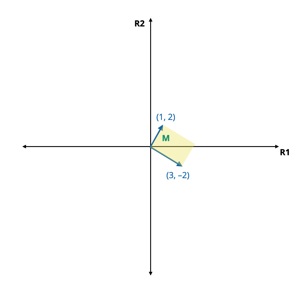
Figure 7.1: Matrix M (yellow) in the 2-dimensional coordinate system defined by R1 and R2.

Because most matrices have much higher dimensions, we typically do not visualize them geometrically. For additional detail on the geometry of matrices, see YouTube content creator 3Blue1Brown’s excellent playlist, Essence of Linear Algebra.

7.0.4 Matrices in R

To enter a matrix in R, we use the matrix() function, similar to creating a vector. The only difference is that the nrow= or ncol= argument will include a value other than 1. The elements of the matrix given in the data= argument, by default, will be filled-in by columns. For example to create matrix B from the earlier example, we can use the following syntax.

# Create B by filling in columns
B = matrix(
  data = c(5, 7, -2, 1, 3, -1),
  nrow = 3,
  ncol = 2
  )

# Display B
B

     [,1] [,2]
[1,]    5    1
[2,]    7    3
[3,]   -2   -1

The byrow=TRUE argument will fill the elements by rows rather than columns.

# Create B by filling in rows
B = matrix(
  data = c(5, 1, 7, 3, -2, -1),
  byrow = TRUE,
  nrow = 3
  )

# Display B
B

     [,1] [,2]
[1,]    5    1
[2,]    7    3
[3,]   -2   -1

The dim() function can be used to return the dimensions of a matrix.

# Get matrix dimensions
dim(B)

[1] 3 2

Lastly, we can index elements of a matrix by specifying the row and column number of the matrix object for the element we want in square brackets. These values are separated by a comma. For example, to index the element in B that is in the 2nd row and 1st column, we use the following syntax:

# Index the element in the 2nd row, 1st column
B[2, 1]

[1] 7

7.1 Matrix Equality

Two matrices are said to be equal if they satisfy two conditions:

They have the same dimensions, and
All corresponding elements are equal.

Consider the following matrices:

\[ \mathbf{A} = \begin{bmatrix} 112 & 86 & 0 \\ 134 & 94 & 0 \end{bmatrix} \qquad \mathbf{B} = \begin{bmatrix} 112 & 134 \\86 & 94 \\ 0 & 0 \end{bmatrix} \qquad \mathbf{C} = \begin{bmatrix} 112 & 86 & 0 \\ 134 & 94 & 0 \end{bmatrix} \]

Within this set of matrices,

\(\mathbf{A} \neq \mathbf{B}\), since they do not have the same dimensions. A is a \(2\times3\) matrix and B is a \(3\times2\) matrix.
Similarly, \(\mathbf{A} \neq \mathbf{B}\), they also do not have the same dimensions.
\(\mathbf{A} = \mathbf{C}\) since both matrices have the same dimensions and all corresponding elements are equal.

7.2 Exercises

Consider the following matrices:

\[ \mathbf{A} = \begin{bmatrix}5 & 6 & 4& 5 & 9 \\21 & 23 & 24 & 22 & 20 \end{bmatrix} \qquad \mathbf{b}^\intercal = \begin{bmatrix}0 & 1 & 0 & 0 \end{bmatrix} \qquad \mathbf{Y} = \begin{bmatrix}2 & 3 & 1 \\5 & 6 & 8\\9 & 4 & 7 \end{bmatrix} \]

Use notation to describe the dimensions of A.

Use notation to describe the dimensions of b.

Use notation to describe the dimensions of Y.

The matrix X contains data from four students’ of four different course exams.

\[ \mathbf{X} = \begin{bmatrix}32 & 54 & 56 & 21 \\42 & 23 & 52 & 35 \\ 16 & 41 & 54 & 56 \\ 58 & 52 & 31 & 24 \end{bmatrix} \]

Which student obtained a 35 and on which test? Report the row and column using subscript notation.

Using subscript notation, indicate the 4th student’s score on the 1st exam.

In computation, a matrix is a very particular type of data structure in which every column has the same type of data (e.g., every column is numeric, or every column is a character variable). A data frame is a more generalized computational structure that accommodates multiple types of columns. In some computational languages this structure is referred to as a data matrix.↩︎