Chapter 18 Systems of Equations

One thing that matrix algebra is really useful for is solving systems of equations. For example, consider the following system of two equations:

\[ \begin{split} 3x + 4y &= 10 \\[2ex] 2x + 3y &= 7 \end{split} \]

The set of equations is referred to as a system of equations, and “solving” this system of equations is akin to determining the values of x and y that satisfy all equations in the system. In an algebra class, you may have learned to solve these equations by graphing them, using substitution, or elimination. Based on these methods we would find that \(x=2\) and \(y=1\). Since this system has a solution, we say the system of equations is consistent.

If this were the only set of x- and y-values that could simultaneously solve all of the equations, then this consistent system is said to have a unique solution. In other systems of equations, there may be an infinite number of x- and y-values that provide solutions (referred to as a dependent system of equations) or no x- and y-values that offer a solution (an inconsistent system of equations).

Graphically, a consistent system of equations with a unique solution intersect at a unique point. In our example, the two lines defined by the equations would intersect at the point \((2,1)\). If the system of equations were dependent, the two equations would form the same line. For example,

\[ \begin{split} x + y &= 6 \\[2ex] 2x + 2y &= 12 \end{split} \]

In this example, every \((x,y)\) value that lies on the two lines is a potential solution for the system; and there are an infinite number of these solutions. In an inconsistent system of equations, the two lines do not intersect; they are parallel.⁹ For example, the following system of equations is inconsistent:

\[ \begin{split} x + y &= 5 \\[2ex] x + y &= 10 \end{split} \]

These two lines are parallel (do not intersect), so there is not any values of x and y that satisfy both equations. Note that the second equation in the system has been changed disproportionately from the first; namely the left-side of the first equation was multiplied by one to obtain the left-side of the second equation and the right-side of the first equation was multiplied by two. Algebraically, inconsistent systems share this characteristic that one side of the equation has been disproportionately changed from the other side.

18.1 Solving Systems of Equations with Matrix Algebra

We can also use matrix algebra to solve systems of equations. To do this, we will re-visit the earlier system of equations:

\[ \begin{split} 3x + 4y &= 10 \\[2ex] 2x + 3y &= 7 \end{split} \]

We first need to write this system of equations using matrices. Because there are two equations, we can initially formulate each side of the equality as a \(2 \times 1\) matrix:

\[ \begin{bmatrix} 3x + 4y \\ 2x + 3y \end{bmatrix} = \begin{bmatrix} 10 \\ 7 \end{bmatrix} \]

Now, we can re-write the left-hand side of the equality as the product of two matrices:

\[ \begin{bmatrix} 3 & 4 \\ 2 & 3 \end{bmatrix}\begin{bmatrix} x \\ y \end{bmatrix} = \begin{bmatrix} 10 \\ 7 \end{bmatrix} \]

Note that the elements of the “left” (premultiplied) matrix on the left-hand side of the equality are composed of the four coefficients that make up the system of equations. The “right” (postmultiplied) matrix on the left-hand side of the equality is a column matrix composed of the unknowns in the original system of equations. The matrix on the right-hand side of the equality is a column matrix made up of the equality values in the original system of equations.

Note that the matrix multiplication on the left-hand side of the equality is defined and produces the appropriately dimensioned matrix on the right-hand side of the equality.

\[ \underset{2\times 2}{\begin{bmatrix} 3 & 4 \\ 2 & 3 \end{bmatrix}}\underset{2\times 1}{\begin{bmatrix} x \\ y \end{bmatrix}} = \underset{2\times 1}{\begin{bmatrix} 10 \\ 7 \end{bmatrix}} \]

If we use a more general notation,

\[ \underset{n\times n}{\mathbf{A}}~\underset{n\times 1}{\mathbf{X}} = \underset{n\times 1}{\mathbf{C}} \]

where n is the number of equations (and unknowns) in the system, A is a matrix representing the coefficients associated with each of the unknowns in the system equations, and C is the matrix representing the scalar equality values.

To solve this general equation, we premultiply both sides of the equation by \(\mathbf{A}^{-1}\).

\[ \mathbf{A}^{-1}\mathbf{A}\mathbf{X} = \mathbf{A}^{-1}\mathbf{C} \]

This will result in

\[ \begin{split} (\mathbf{A}^{-1}\mathbf{A})\mathbf{X} &= \mathbf{A}^{-1}\mathbf{C} \\[2ex] \mathbf{I}\mathbf{X} &= \mathbf{A}^{-1}\mathbf{C} \\[2ex] \mathbf{X} &= \mathbf{A}^{-1}\mathbf{C} \end{split} \]

Thus, we can solve for the elements in X (x and y) by premultiplying C by the inverse of A. In our example,

\[ \begin{split} \overset{\mathbf{A}}{\begin{bmatrix} 3 & 4 \\ 2 & 3 \end{bmatrix}}\overset{\mathbf{X}}{\begin{bmatrix} x \\ y \end{bmatrix}} &= \overset{\mathbf{C}}{\begin{bmatrix} 10 \\ 7 \end{bmatrix}} \\[2ex] \overset{\mathbf{A}^{-1}}{\begin{bmatrix} 3 & -4 \\ -2 & 3 \end{bmatrix}}\overset{\mathbf{A}}{\begin{bmatrix} 3 & 4 \\ 2 & 3 \end{bmatrix}}\overset{\mathbf{X}}{\begin{bmatrix} x \\ y \end{bmatrix}} &= \overset{\mathbf{A}^{-1}}{\begin{bmatrix} 3 & -4 \\ -2 & 3 \end{bmatrix}}\overset{\mathbf{C}}{\begin{bmatrix} 10 \\ 7 \end{bmatrix}} \\[2ex] \overset{\mathbf{I}}{\begin{bmatrix} 1 & 0 \\ 0 & 1 \end{bmatrix}}\overset{\mathbf{X}}{\begin{bmatrix} x \\ y \end{bmatrix}} &= \overset{\mathbf{A}^{-1}\mathbf{C}}{\begin{bmatrix} 2 \\ 1 \end{bmatrix}} \\[2ex] \overset{\mathbf{X}}{\begin{bmatrix} x \\ y \end{bmatrix}} &= \overset{\mathbf{A}^{-1}\mathbf{C}}{\begin{bmatrix} 2 \\ 1 \end{bmatrix}} \\[2ex] \end{split} \]

Because the two matrices here, \(\mathbf{X}\) and \(\mathbf{A}^{-1}\mathbf{C}\), are equal, all of the elements in the same position are equal. Thus \(x=2\) and \(y=1\).

18.1.1 Solving this System of Equations Using R

We can use R to carry out this matrix algebra.

# Create A
A = matrix(
  data = c(3, 2, 4, 3),
  nrow = 2
)


# Create C
C = matrix(
  data = c(10, 7),
  nrow = 2
)


# Solve for X
solve(A) %*% C

     [,1]
[1,]    2
[2,]    1

What happens when we try to solve for a consistent system of equations that have an infinite number of solutions? Using our example from above:

# Create A
A = matrix(
  data = c(1, 2, 1, 2),
  nrow = 2
)


# Create C
C = matrix(
  data = c(6, 12),
  nrow = 2
)


# Solve for X
solve(A) %*% C

Error in solve.default(A): Lapack routine dgesv: system is exactly singular: U[2,2] = 0

We cannot solve this system of equations because the inverse of A is singular (the determinant of A is zero). What happens when we try to solve for a dependent system of equations? Using our example from above:

# Create A
A = matrix(
  data = c(1, 1, 1, 1),
  nrow = 2
)


# Create C
C = matrix(
  data = c(5, 10),
  nrow = 2
)


# Solve for X
solve(A) %*% C

Error in solve.default(A): Lapack routine dgesv: system is exactly singular: U[2,2] = 0

We also cannot solve this system of equations because the inverse of A is singular (the determinant of A is zero).

18.2 Linear Dependence and Independence

We recognize that when a redundant equation is present in a system of equations, the matrix of coefficients (A) is singular, the determinant is zero. This is one definition of a linearly dependent system of equations. When none of the equations in a system are redundant with any other equation within the system, the system of equations is linearly independent.

Consider a vector z where \(\mathbf{z} = a\mathbf{x} + b\mathbf{y}\). That is, z is a linear function of the vectors x and y. (We could also say z is linearly dependent on x and y.) When we have used vector addition or vector subtraction, we were actually creating linear combinations of vectors where the scalars were all equal to \(+1\) or \(–1\). For example, \(\mathbf{z} = \mathbf{x} + \mathbf{y}\) is mathematically equivalent to \(\mathbf{z} = 1\mathbf{x} + 1\mathbf{y}\). In this case, the coefficients for x and y are both \(+1\); \(a=1\) and \(b=1\).

Formally, a set of vectors, \(\mathbf{a}_1, \mathbf{a}_2, \ldots \mathbf{a}_n\), is linearly dependent if there exists a set of scalars (not all zero) where:

\[ c_1\mathbf{a}_1 + c_2 \mathbf{a}_2 + \ldots + c_n\mathbf{a}_n = 0 \] If no set of scalars exist to satisfy this condition, the set of vectors is linearly independent. For the above condition to be true, at least one of the vectors must be redundant with another, it can be expressed as a linear combination of the others. Linear dependence implies redundancy among at least two of the vectors. For example consider the following three vectors:

\[ \mathbf{x} = \begin{bmatrix}4\\6\end{bmatrix} \qquad \mathbf{y}= \begin{bmatrix}2\\1\end{bmatrix} \qquad \mathbf{z}= \begin{bmatrix}6\\11\end{bmatrix} \]

These three vectors can be written as:

\[ \begin{split} 2\mathbf{x} - 1 \mathbf{y} -1 \mathbf{z} &= 0 \\[2ex] 2\begin{bmatrix}4\\6\end{bmatrix} - 1 \begin{bmatrix}2\\1\end{bmatrix} - 1 \begin{bmatrix}6\\11\end{bmatrix} &= 0 \end{split} \]

Since we have a set of scalars \(\{2,-1,-1\}\) that satisfy this equation where none of the scalars are zero, this system of equations is linearly dependent.

18.3 Singularity

Recall that in a singular matrix, the determinant if the matrix is zero. A matrix that is singular implies that one or more of the rows (or columns) is linearly dependent; there exists a set of scalars that satisfies our definition. Earlier we saw that:

\[ \mathbf{A} = \begin{bmatrix}1 & 1 \\ 2 & 2\end{bmatrix} \]

was singular. Namely,

\[ \begin{split} \vert\mathbf{A}\vert &= 1(2) - 2(1) \\[2ex] &= 0 \end{split} \] We can also find scalars \(c_1\) and \(c_2\) such that the row vectors (or column vectors) of A can be written as \(c_1\mathbf{a}_1 + c_2 \mathbf{a}_2 = 0\). Using the two row vectors:

\[ \begin{split} 2\begin{bmatrix}1\\1\end{bmatrix} - 1 \begin{bmatrix}2\\2\end{bmatrix} &= 0 \\[2ex] 2\mathbf{a}_1 - 1 \mathbf{a}_2 &= 0 \end{split} \]

In general, when A is singular the rows are linearly dependent. The columns are similarly linearly dependent when A is singular.

There is a theorem in linear algebra that suggests that any n-element vector can be written as a linear combination of n linearly independent n-element vectors. Finding such vectors can be difficult, but we rely on this theorem in statistics.

18.4 Rank of a Matrix

The column rank of a matrix describes the dimensionality of the column space for that matrix, and the row rank describes the dimensionality of the row space for that matrix. It turns out that the column and row ranks of a matrix are the same, so we just refer to the dimensionality, or rank of a matrix. Because dimensionality is related to the independence of the rows/columns, the rank of a matrix is also the number of rows or columns that are linearly independent:

\[ \mathrm{Rank}(\mathbf{A}) = \begin{cases}\mathrm{number~of~linearly~independent~rows~of~}\mathbf{A} \\ \mathrm{number~of~linearly~independent~columns~ of~}\mathbf{A}\end{cases} \]

For an \(n \times p\) dimensional matrix A, the maximum possible rank is the smaller value of n and p. That is,

\[ 0 \leq \mathrm{Rank}(\underset{n\times p}{\mathbf{A}}) \leq \min(n,p) \]

The rank of a matrix would be zero only if the matrix were a null matrix. For all other matrices, the minimum possible rank would be one.

When all of the row and column vectors in a matrix are linearly independent the matrix is said to be of full rank. That is, when the rank of A is the maximum possible rank, it is of full rank. When the rank of A is smaller than both n and p, the matrix is said to be of deficient rank. This implies that at least one of the row (or column) vectors is linearly dependent. It turns out only a square matrix can be of full rank—rectangular matrices will always have a rank less than either n or p.

For example, consider the following matrices:

\[ \mathbf{A} = \begin{bmatrix}3 & 5 \\ 1 & 2\end{bmatrix} \qquad \mathbf{B} = \begin{bmatrix}1 & 3 & 5 \\ 1 & 2 & 3 \\ 2 & 5 & 8\end{bmatrix} \]

The rank of A is 2, since the two ro vectors (or the two column vectors) are linearly independent. Since 2 is the maximum possible rank of a \(2 \times 2\) matrix, we consider A to be of full rank. Matrix B, on the other hand, is of deficient rank. This is because the rank of B is 2, which is less than the maximum possible rank of 3 for a \(3\times 3\) matrix. This means that two of the three rows (or columns) of B are linearly independent. It turns out the third row of B is a linear combination of the first and second rows:

\[ \overset{\mathrm{Row~3}}{\begin{bmatrix}2 & 5 & 8\end{bmatrix}} = \overset{\mathrm{Row~1}}{\begin{bmatrix}1 & 3 & 5\end{bmatrix}} + \overset{\mathrm{Row~2}}{\begin{bmatrix}1 & 2 & 3\end{bmatrix}} \]

We can compute the rank of a matrix by using the rankMatrix() function from the Matrix package.

# Create A
A = matrix(
  data = c(3, 5, 1, 2),
  byrow = TRUE,
  ncol = 2
)

# Compute rank of A
Matrix::rankMatrix(A)

[1] 2
attr(,"method")
[1] "tolNorm2"
attr(,"useGrad")
[1] FALSE
attr(,"tol")
[1] 4.440892e-16

# Create B
B = matrix(
  data = c(1, 3, 5, 1, 2, 3, 2, 5, 8),
  byrow = TRUE,
  ncol = 3
)

# Compute rank of B
Matrix::rankMatrix(B)

[1] 2
attr(,"method")
[1] "tolNorm2"
attr(,"useGrad")
[1] FALSE
attr(,"tol")
[1] 6.661338e-16

The determinant of a matrix also gives us insight into whether a matrix is of full rank. Singular matrices (determinant = 0) are of deficient rank, while non-singular matrices are of full rank.

# Compute determinant
det(A)

[1] 1

# Compute determinant
det(B)

[1] 0

All of this implies that if A is non-singular (\(\lvert \mathbf{A} \rvert \neq 0\)), then:

• A has an inverse;
• \(\mathrm{rank}(\mathbf{A}) = n\), or A is full rank;
• All rows of A are linearly independent; and
• All columns of A are linearly independent.

18.5 Rank and the Solution of Systems of Equations

Remember, our goal was to use matrix algebra to solve a system of equations. In order to do this we need to evaluate the independence of the system of equations. Consider the following system of equations:

\[ \begin{split} x_1 + x_2 + x_3 &= 5 \\[2ex] 2x_1 – 1x_2 + 6x_3 &= 12 \\[2ex] x_1 + 3x_2 + 5x_3 &= 17 \end{split} \] The coefficient matrix (\(\mathbf{A}\)) and the augmented coefficient matrix (\(\mathbf{A}\vert \mathbf{c}\)) are:

\[ \mathbf{A} = \begin{bmatrix} 1 & 1 & 1 \\ 2 & – 1 & 6\\ 1 & 3 & 5 \end{bmatrix} \qquad \mathbf{A}\vert \mathbf{c} = \begin{bmatrix} 1 & 1 & 1 & 5\\ 2 & – 1 & 6 & 12\\ 1 & 3 & 5 & 17 \end{bmatrix} \]

Note that the augmented coefficient matrix is simply the coefficient matrix with an appended column that include the solutions from the system of equations (the c vector from \(\mathbf{Ax}=\mathbf{c}\)).

A theorem in linear algebra states that a system of equations is independent (consistent) if the rank of the coefficient matrix is the same as the rank of the augmented coefficient matrix, \(\mathrm{rank}(\mathbf{A}) = \mathrm{rank}(\mathbf{A}\vert \mathbf{c})\). Examining the rank of A, we find:

Computing the rank of A:

# Create A
A = matrix(
  data = c(1, 1, 1, 2, -1, 6, 1, 3, 5),
  byrow = TRUE,
  ncol = 3
)

# Create A|y
A_y = matrix(
  data = c(1, 1, 1, 5, 2, -1, 6, 12, 1, 3, 5, 17),
  byrow = TRUE,
  ncol = 4
)

# Compute rank of A
Matrix::rankMatrix(A)

[1] 3
attr(,"method")
[1] "tolNorm2"
attr(,"useGrad")
[1] FALSE
attr(,"tol")
[1] 6.661338e-16

# Compute rank of A|y
Matrix::rankMatrix(A_y)

[1] 3
attr(,"method")
[1] "tolNorm2"
attr(,"useGrad")
[1] FALSE
attr(,"tol")
[1] 8.881784e-16

The rank of A is 3, which means A is of full rank. This also implies that A is non-singular (\(\lvert \mathbf{A}\rvert \neq 0\)), and that A has an inverse. Furthermore, since the rank of \(\mathbf{A}\vert \mathbf{c}\) is also 3, the system of equations is consistent (linearly independent). This means that we can solve the equations using:

\[ \begin{split} \mathbf{x} &= \mathbf{A}^{-1}\mathbf{y}\\[2ex] \begin{bmatrix} x_1 \\ x_2\\ x_3 \end{bmatrix} &= \begin{bmatrix} 1 & 1 & 1 \\ 2 & – 1 & 6\\ 1 & 3 & 5 \end{bmatrix}^{-1} \begin{bmatrix} 5 \\ 12\\ 17 \end{bmatrix} \end{split} \]

Computing this, we find \(x_1 = 1\), \(x_2=2\), and \(x_3=2\).

# Create y
y = matrix(
  data = c(5, 12, 17),
  ncol = 1
)

# Solve system of equations
solve(A) %*% y

     [,1]
[1,]    1
[2,]    2
[3,]    2

Another theorem of linear algebra provides a way to evaluate whether a consistent set of equations has an infinite number of solutions. A consistent system of n equations in n unknowns has a unique solution if the rank of the coefficient matrix is equal to its order, that is \(\mathrm{rank}(\mathbf{A}) = n\).

In the example, there are three equations and three unknowns and the rank of the coefficient matrix, A, is 3. The solution we have computed is unique. Another way to state this is: A consistent system of equations where A is of order n has a unique solution if and only if \(\mathbf{A}^{-1}\) exists. This is important in applications where we have the same number of unknowns as equations.

When the number of equations equals the number of unknowns, and \(\lvert \mathbf{A} \rvert \neq 0\), there is a unique solution. That is, when A is full rank, a unique solution exists for \(\mathbf{Ax} = \mathbf{y}\). This is true because:

1. If \(\lvert \mathbf{A} \rvert \neq 0\), then \(\mathrm{rank}(\mathbf{A}) = n\).
2. If \(\mathrm{rank}(\mathbf{A} \vert \mathbf{c}) = \mathrm{rank}(\mathbf{A})\), the equations are consistent.
3. If the equations are consistent and \(\mathrm{rank}(\mathbf{A}) = n\), there is a unique solution.

Figure 18.1 shows a flowchart that you can use to determine whether a system of equations is consistent or not, and if so, whether there is a unique solution or whether it has an infinite number of solutions.

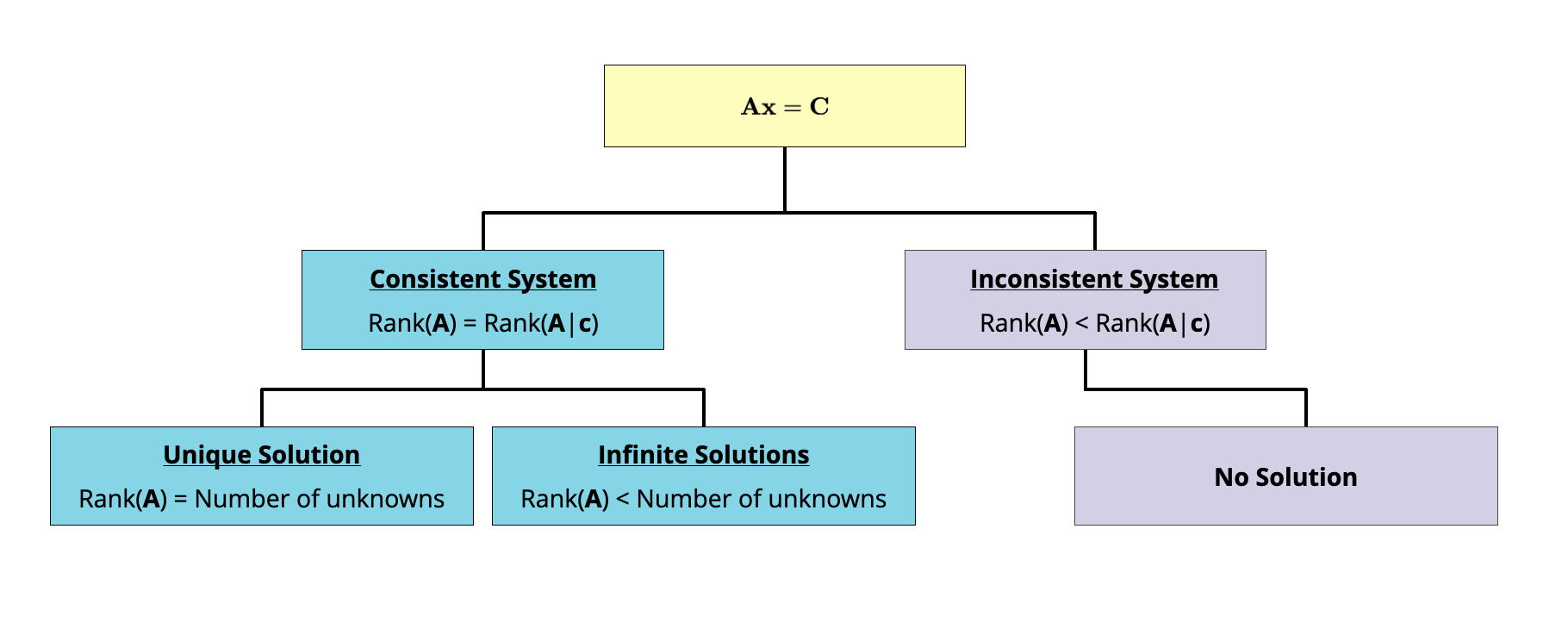
Figure 18.1: Flowchart to determine whether a system of equations is consistent or not, and how many solutions exist.

18.6 Exercises

Consider the following matrices:

\[ \mathbf{A} = \begin{bmatrix}1 & 0 & 0 \\0 & 1 & 0 \\0 & 0 & 1 \end{bmatrix} \qquad \mathbf{B} = \begin{bmatrix}1 & 2 & 3\\4 & 5 & 6\\7 & 8 & 9 \end{bmatrix} \qquad \mathbf{C} = \begin{bmatrix}2 & 3 & 8 \\15 & 5 & 9\\6 & 9 & 24 \end{bmatrix} \]

1. Determine which of the matrices (A, B, and C) have linearly independent rows and which have linearly dependent rows.

• All rows in A are linearly independent, since it has a rank of 3.
• The rank of B is 2, which implies that there is a linearly dependent row. There are a number of other ways to represent this dependency. For example, \(\mathrm{Row~3} = 2(\mathrm{Row~2}) - 1(\mathrm{Row~1})\).
• The rank of C is also 2, which implies that there is a linearly dependent row. There are a number of other ways to represent this dependency. For example, \(\mathrm{Row~3} = 3(\mathrm{Row~2}) + 0(\mathrm{Row~1})\).

Consider the following system of equations:

\[ \begin{split} 2(x_1) + x_2 &= 6 \\[2ex] x_1 + 3(x_2) &= 8 \end{split} \] 2. Write out the coefficient matrix (A) and the augmented coefficient matrix (\(\mathbf{A} \vert \mathbf{c}\)).

\[ \mathbf{A} = \begin{bmatrix}2 & 1 \\ 1 & 3 \end{bmatrix} \qquad \mathbf{A} \vert \mathbf{c} = \begin{bmatrix}2 & 1 & 6 \\ 1 & 3 & 8 \end{bmatrix} \]

3. Use the ranks of \(\mathbf{A}\) and \(\mathbf{A} \vert \mathbf{c}\) to determine whether the system of equations is consistent.

The ranks of the two matrices are:

• \(\mathrm{Rank}(\mathbf{A}) = 2\)
• \(\mathrm{Rank}(\mathbf{A} \vert \mathbf{c}) = 2\)

Since the rank of the coefficient matrix and the augmented coefficient matrix are equal, the system of equations is consistent.

4. Based on the rank of the coefficient matrix, will there be a unique solution to the system of equations?

Since A is of full rank, the solution will be unique.

5. Use R to solve the system of equations.

# Create A
A = matrix(
  data = c(2, 1, 1, 3), 
  ncol = 2
  )

# Create y
y = matrix(
  data = c(6, 8),
  ncol = 1
)

# Solve system of equations
solve(A) %*% y

     [,1]
[1,]    2
[2,]    2

Consider the following system of equations:

\[ \begin{split} 25(x_1) + 5(x_2) + x_3 &= 106.8 \\[2ex] 64(x_1) + 8(x_2) + x_3 &= 177.2 \\[2ex] 89(x_1) + 13(x_2) + 2(x_3) &= 284.0 \\[2ex] \end{split} \] 6. Use R to compute the determinant of the coefficient matrix. Based on the determinant, will there be a unique solution to the system of equations?

# Create A
A = matrix(
  data = c(25, 5, 1, 64, 8, 1, 89, 13, 2), 
  byrow = TRUE,
  ncol = 3
  )

# Compute determinant
det(A)

[1] 0

Since A is singular, there is not a unique solution to the system of equations. (The rank of the coefficient matrix and the augmented coefficient matrix are both 2, so the system is consistent. And, since there is no unique solution, this means there are an infinite number of solutions.)

---

9. Another way to think about dependent systems of equations is that they are redundant.↩︎