
Chapter 13 Properties of Square Matrices
In this chapter, you will learn about several properties of square matrices encountered in statistical and psychometric applications. These properties are also useful for computation.
13.1 Matrix Trace
The trace of a square matrix is the sum of the elements along the main diagonal.8 For example, consider the matrix Y:
\[ \underset{3\times 3}{\mathbf{Y}} = \begin{bmatrix} \color{red}0 & 1 & 0 \\ 1 & \color{red}3 & -8\\ 10 & 4 & \color{red}{-2} \end{bmatrix} \]
The trace of Y is \(0 + 3 + -2 = 1\). To compute the trace using R, we use the sum() and diag() functions.
# Create matrix
Y = matrix(
  data = c(0, 1, 0, 1, 3, -8, 10, 4, -2),
  byrow = TRUE,
  ncol = 3
  )

# Compute trace of Y
sum(diag(Y))
[1] 1You can also use the tr() function from the psych library to compute the trace.
library(psych)
tr(Y)
[1] 113.2 Determinant
Every square matrix has a unique scalar value associated with it, called the determinant. The determinant, denoted by \(\left| \mathbf{A} \right|\) or \(\mathrm{det}(\mathbf{A})\), has many uses in statistical and psychometric applications. For example, the determinant of a variance-covariance matrix provides information about the generalized variance of several variables. It is also useful for computing several multivariate statistics.
We will illustrate the process for calculating the determinant for a \(1 \times 1\), \(2 \times 2\), and \(3 \times 3\) matrix. Beyond a \(3 \times 3\) matrix the determinant is more difficult to calculate, and those methods will not be discussed here. In practice, computation is used to find the determinant.
13.2.1 Determinant for a \(1 \times 1\) matrix.
The determinant of a \(1 \times 1\) scalar matrix is equal to the scalar, namely \(\mathrm{det}\big([a_1]\big) = a_1\). For example, consider the scalar matrix having an element of \(-1\):
\[ \begin{vmatrix}-1\end{vmatrix} = -1 \]
The determinant of this matrix is \(-1\).
13.2.2 Determinant for a \(2 \times 2\) matrix.
The determinant of the \(2\times 2\) matrix A, given as
\[ \underset{2\times 2}{\mathbf{A}} = \begin{bmatrix} a_{11} & a_{12} \\ a_{21} & a_{22} \end{bmatrix} \]
is the scalar \(a_{11}(a_{22}) - a_{12}(a_{21})\). That is, we are taking the product of the elements along the main diagonal (shown in pink below) and subtracting the product of the elements on the off diagonal (shown in blue below).
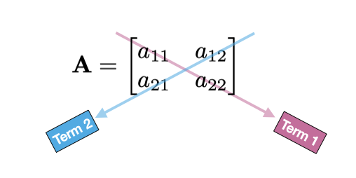
Figure 13.1: Procedure for finding the product terms in the determinant for a 2x2 matrix. The first term is computed by multiplying the elements along the pink arrow, and the second term is computed by multiplying the elements along the blue arrow.
Color-coding the formula:
\[ \begin{split} \mathrm{det}(\mathbf{A}) = ~&\color{#CC79A7}{\overbrace{a_{11}(a_{22})}^\mathrm{Term~1}} - \color{#56B4E9}{ \overbrace{a_{12}(a_{21})}^\mathrm{Term~2} } \end{split} \]
As an example, consider the matrix Y:
\[ \mathbf{Y} = \begin{bmatrix} 1 & 2 \\ 3 & 4 \end{bmatrix} \]
The determinant of Y is:
\[ \begin{split} \mathrm{det}(\mathbf{Y}) &= \begin{vmatrix} 1 & 2 \\ 3 & 4 \end{vmatrix} \\[2ex] &= 1(4) - 2(3) \\[2ex] &= -2 \end{split} \]
13.2.3 Determinant for a \(3 \times 3\) matrix.
The determinant of a \(3\times 3\) matrix A, where
\[ \underset{3\times 3}{\mathbf{A}} = \begin{bmatrix} a_{11} & a_{12} & a_{13} \\ a_{21} & a_{22} & a_{23} \\ a_{31} & a_{32} & a_{33} \end{bmatrix} \]
is defined as:
\[ \begin{split} \mathrm{det}(\mathbf{A}) = &a_{11}(a_{22})(a_{33}) + a_{12}(a_{23})(a_{31}) + a_{13}(a_{21})(a_{32}) -\\ &a_{13}(a_{22})(a_{31}) - a_{11}(a_{23})(a_{32}) - a_{12}(a_{21})(a_{33}) \end{split} \]
Although this looks complicated the procedure for finding this is easily described. Write out the matrix A and additionally append the first two columns to the right of the matrix. These additional columns are shown in red below.
\[ \mathbf{A} = \begin{bmatrix} a_{11} & a_{12} & a_{13} \\ a_{21} & a_{22} & a_{23} \\ a_{31} & a_{32} & a_{33} \end{bmatrix} \color{red}{\begin{matrix}a_{11} & a_{12} \\ a_{21} & a_{22} \\ a_{31} & a_{32} \end{matrix}} \]
The first three product terms in the determinant are computed by: multiplying the elements found in the main diagonal (first product term), and the elements in the remaining two parallel diagonals (shown in pink below). Similarly, the second set of three products are found by multiplying the elements in the opposite diagonal and the elements in the two parallel diagonals (shown in blue below).
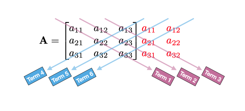
Figure 13.2: Procedure for finding the product terms in the determinant for a 3x3 matrix. The first three terms computed by multiplying the elements along each of the pink arrows, and the second set of three terms are computed by multiplying the elements along each of the blue arrows.
We add together the first three product terms and subtract the last three product terms. This gives us the determinant.
\[ \begin{split} \mathrm{det}(\mathbf{A}) = ~&\color{#CC79A7}{\overbrace{a_{11}(a_{22})(a_{33})}^\mathrm{Term~1} + \overbrace{a_{12}(a_{23})(a_{31})}^\mathrm{Term~2} + \overbrace{a_{13}(a_{21})(a_{32})}^\mathrm{Term~3}} \color{#56B4E9}{-}\\ &\color{#56B4E9}{\underbrace{a_{13}(a_{22})(a_{31})}_\mathrm{Term~4} - \underbrace{a_{11}(a_{23})(a_{32})}_\mathrm{Term~5} - \underbrace{a_{12}(a_{21})(a_{33})}_\mathrm{Term~6}} \end{split} \]
As an example consider the following \(3 \times 3\) matrix:
\[ \underset{3\times 3}{\mathbf{X}} = \begin{bmatrix} 3 & 5 & 0 \\ 1 & 2 & 1 \\ 3 & 6 & 4 \end{bmatrix} \]
The determinant of X is:
\[ \begin{split} \mathrm{det}(\mathbf{X}) &= \begin{vmatrix} 3 & 5 & 0 \\ 1 & 2 & 1 \\ 3 & 6 & 4 \end{vmatrix} \\[2ex] &= 3(2)(4) + 5(1)(3) + 0(1)(6) - 0(2)(3) - 3(1)(6) - 5(1)(4) \\[2ex] &= 24 + 15 + 0 - 0 - 18 - 20 \\[2ex] &= 1 \end{split} \]
13.2.4 Using R to Find the Determinant
We can use the det() function to compute the determinant, using R. Below we use this function to compute the determinant for each of the matrices given in the examples above.
# Create matrix
Y = matrix(
  data = c(1, 2, 3, 4),
  byrow = TRUE,
  ncol = 2
)

# Find determinant
det(Y)
[1] -2# Create matrix
X = matrix(
data = c(3, 5, 0, 1, 2, 1, 3, 6, 4),
byrow = TRUE,
ncol = 3
)
# Find determinant
det(X)[1] 113.2.5 Properties of the Determinant
There are several useful properties of the determinant. For each of these properties A and B are matrices and \(\lambda\) is a scalar.
- If every element in a row (or column) of a matrix is zero, then the determinant of that matrix is zero.
- If two rows (or columns) of a matrix are swapped, the determinant changes sign.
- If two rows (or columns) of a matrix are identical, the determinant of that matrix is zero.
- \(\mathrm{det}(\mathbf{A}) = \mathrm{det}(\mathbf{A}^\intercal)\)
- If \(\mathbf{B}=\lambda\mathbf{A}\), then \(\mathrm{det}(\mathbf{B}) = \lambda\big(\mathrm{det}(\mathbf{A})\big)\).
- For an \(n \times n\) matrix A, \(\mathrm{det}(\lambda\mathbf{A}) = \lambda^n\big(\mathrm{det}(\mathbf{A})\big)\).
- If A and B are of the same order, \(\mathrm{det}(\mathbf{A})\mathrm{det}(\mathbf{B}) = \mathrm{det}(\mathbf{AB})\)
13.3 Matrix Inverse
The inverse of a \(n \times n\) matrix A, denoted \(\mathbf{A}^{-1}\), is also a \(n \times n\) matrix having the property that:
\[ \mathbf{A}\mathbf{A}^{-1} = \mathbf{A}^{-1}\mathbf{A} = \mathbf{I} \]
That is, when we postmultiply (or premultiply) a square matrix by its inverse, we obtain the \(n \times n\) identity matrix. Not all square matrices have an inverse. If a square matrix has an inverse we say that it is invertible or nonsingular.
Typically, we will use the computer to find a matrix’s inverse. However, for the \(2\times2\) matrix, we can describe a procedure that can be used to find the inverse. To find \(\mathbf{A}^{-1}\) we:
- Compute the determinant of A.
- Create a new matrix, call it B where we swap the elements on the main diagonal of A and change the signs on the off diagonals elements.
- Multiply B by the reciprocal of the determinant.
As an example, consider the following \(2 \times 2\) matrix:
\[ \mathbf{A} = \begin{bmatrix} 2 & 1 \\ 1 & 3 \end{bmatrix} \]
The determinant of A is 5. Swapping the elements on the main diagonal of A and changing the signs on the off diagonals elements, we get:
\[ \begin{bmatrix} 3 & -1 \\ -1 & 2 \end{bmatrix} \]
To obtain the inverse, we multiply this converted matrix by the reciprocal of the determinant:
\[ \begin{split} \mathbf{A}^{-1} &= \frac{1}{5} \begin{bmatrix} 3 & -1 \\ -1 & 2 \end{bmatrix} \\[2ex] &= \begin{bmatrix} \frac{3}{5} & -\frac{1}{5} \\ -\frac{1}{5} & \frac{2}{5} \end{bmatrix} \end{split} \]
If we postmultiply (or premultiply) this matric by A, we should get the \(2 \times 2\) identity matrix.
\[ \begin{split} \mathbf{A}\mathbf{A}^{-1} &= \begin{bmatrix} 2 & 1 \\ 1 & 3 \end{bmatrix}\begin{bmatrix} \frac{3}{5} & -\frac{1}{5} \\ -\frac{1}{5} & \frac{2}{5} \end{bmatrix} \\[2ex] &= \begin{bmatrix} 1 & 0 \\ 0 & 1 \end{bmatrix} \\[5ex] \mathbf{A}^{-1}\mathbf{A} &= \begin{bmatrix} \frac{3}{5} & -\frac{1}{5} \\ -\frac{1}{5} & \frac{2}{5} \end{bmatrix}\begin{bmatrix} 2 & 1 \\ 1 & 3 \end{bmatrix} \\[2ex] &= \begin{bmatrix} 1 & 0 \\ 0 & 1 \end{bmatrix} \end{split} \]
13.3.1 Find the Inverse using R
To find the inverse using R, we can use the solve() function. If you want fractional elements (rather than decimal elements) you can use the fractions() function from the {MASS} package to convert the decimal output to fractions.
# Create matrix
A = matrix(
  data = c(2, 1, 1, 3),
  byrow = TRUE,
  ncol = 2
)

# Find inverse
solve(A)
[,1] [,2]
[1,] 0.6 -0.2
[2,] -0.2 0.4# Find inverse (output as fractions)
MASS::fractions(solve(A)) [,1] [,2]
[1,] 3/5 -1/5
[2,] -1/5 2/5If you get a message that the system is “exactly singular” or “computationally singular”, the matrix does not have an inverse (or it cannot be computed). In this case, we would say that A is not invertible or is singular.
13.3.2 Properties of the Inverse
There are several useful properties of the matrix inverse.
- If \(\mathrm{det}(\mathbf{A})=0\), then A is singular and \(\mathbf{A}^{-1}\) does not exist.
- If the inverse exists for A, there is only one inverse.
- If the inverse exists for A, the inverse also exists for \(\mathbf{A}^\intercal\)
- \((\mathbf{A}^{-1})^{-1} = \mathbf{A}\)
- \((\mathbf{A}^\intercal)^{-1} = (\mathbf{A}^{-1})^\intercal\)
- \((\mathbf{AB})^{-1} = \mathbf{B}^{-1}\mathbf{A}^{-1}\)
- \((\mathbf{A})^{-n} = (\mathbf{A}^{-1})^n\)
- If \(\lambda\) is a non-zero scalar, \((\lambda\mathbf{A})^{-1} = \frac{1}{\lambda}(\mathbf{A}^{-1})\)
- The inverse of a nonsingular diagonal matrix D is also a diagonal matrix. Moreover, the diagonal elements of \(\mathbf{D}^{-1}\) are the reciprocals of the diagonal elements of D.
- The inverse of a nonsingular symmetric matrix is also a symmetric matrix.
13.4 Exercises
For each of the following matrices, calculate (by-hand) the trace, determinant, and inverse. Then use R to check your work.
- \(\mathbf{A} = \begin{bmatrix}2 & 4 \\3 & 6 \end{bmatrix}\)
- \(\mathbf{B} = \begin{bmatrix}2 & -1 \\3 & 3 \end{bmatrix}\)
For each of the following matrices, calculate (by-hand) the trace, and determinant. Then use R to check your work. Also use R to find the inverse.
- \(\mathbf{C} = \begin{bmatrix}2 & -1 & 3 \\3 & 3 & 4\\1 & 2 & 2 \end{bmatrix}\)
- \(\mathbf{D} = \begin{bmatrix}2 & -1 & 3 \\3 & 3 & 4\\5 & 2 & 7 \end{bmatrix}\)
Since rectangular matrices also have a main diagonal, we can also compute the trace of a rectangular matrix. However, in statistical and psychometric applications (e.g., principle components analysis), the trace is primarily computed on square matrices.↩︎