Simulation Process for Evaluating Hypotheses
To illustrate the ideas behind statistical hypothesis testing, imagine you had flipped a coin 100 times and it had produced heads in 64 of those flips. This proportion of .64 (or 64%) heads made you suspicious about whether the coin was fair and you now want to evaluate whether it is fair, or whether it is producing heads too often.
Statistical Hypotheses
To determine whether the coin is fair or not, we will write and evaluate a set of hypotheses about the population. Hypotheses are mathematical statements about population parameters which are often formed based on prior knowledge and theory in the area of content. In the social sciences, we typically write out two hypotheses about the population parameters: the null hypothesis (\(H_0\)), often referred to as a statement of no effect, and the alternative hypothesis (\(H_A\)), often termed the research hypothesis. For example, here are a set of potential hypotheses about our coin:
\[ \begin{split} H_0:~ &\text{The proportion of heads when flipping the coin is equal to 0.50.}\\ H_A:~ &\text{The proportion of heads when flipping the coin is greater than 0.50.} \end{split} \]
There are a few things to notice about these hypotheses:
- The statements are about the proportion of heads (i.e., about a summary measure).
- The statements are about the population (all flips of the coin), not the sample.
- The null hypothesis (\(H_0\)) is a statement of equality (is equal to).
- The alternative hypothesis often indicates the researcher’s belief about the population summary (e.g., we think the coin is producing more heads than tails).
Additionally, statisticians often use the language of mathematics to express these hypotheses. The same hypotheses expressed via the language of mathematics are:
\[ \begin{split} H_0:~ &\pi_{\mathrm{Heads}} = 0.50\\ H_A:~ &\pi_{\mathrm{Heads}} > 0.50 \end{split} \]
The Greek letter pi (\(\pi\)) denotes a population proportion or probability.1 (In symbolic notation for statistical hypotheses, pi is not the mathematical constant of 3.14.) The subscript of “Heads” indicates that we are considering the proportion of heads in all flips of the coin.
You can always write hypotheses descriptively, without resorting to the symbolic notation. If you are comfortable with the mathematical symbols, feel free to use it; the mathematical notation acts as a shorthand to quickly state a hypothesis and define the model used. As you read research articles or take other courses, you will see statistical hypotheses stated in many ways, so it is good to understand that there are many ways to express the same thing.
Model–Simulate–Evaluate
The process we will use for evaluating a hypothesis is:
- Create a model that conforms to the null hypothesis.
- Use the selected model to generate many, many sets of data (Monte Carlo simulation). The results you collect and pool together from these trials will give a picture of the variation you would expect if the null hypothesis is true.
- Evaluate whether the results observed in the actual data (not the simulated data) are compatible with the expected results produced from the null hypothese. This acts as evidence of support (or nonsupport) for the null hypothesis.
To help you remember this process, you can use the more simplistic mnemonic:
- Model
- Simulate
- Evaluate
This may sound like a straight-forward process, but in practice it can actually be quite complex—especially as you are reading research articles and trying to interpret the findings. First off, the model that is selected is often not provided, nor described, explicitly within most research articles. It is often left to the reader to figure out what the assumed model was. At first, this may be quite difficult, but like most tasks, as you gain experience in this course and as you read more research, you find that there are a common set of models that are typically used by researchers.
Model
The model that you use in the Monte Carlo simulation is directly related to the null hypothesis. In our coin flip example, recall that the null hypothesis was:
\[ H_0:~ \pi_{\mathrm{Heads}} = 0.50 \]
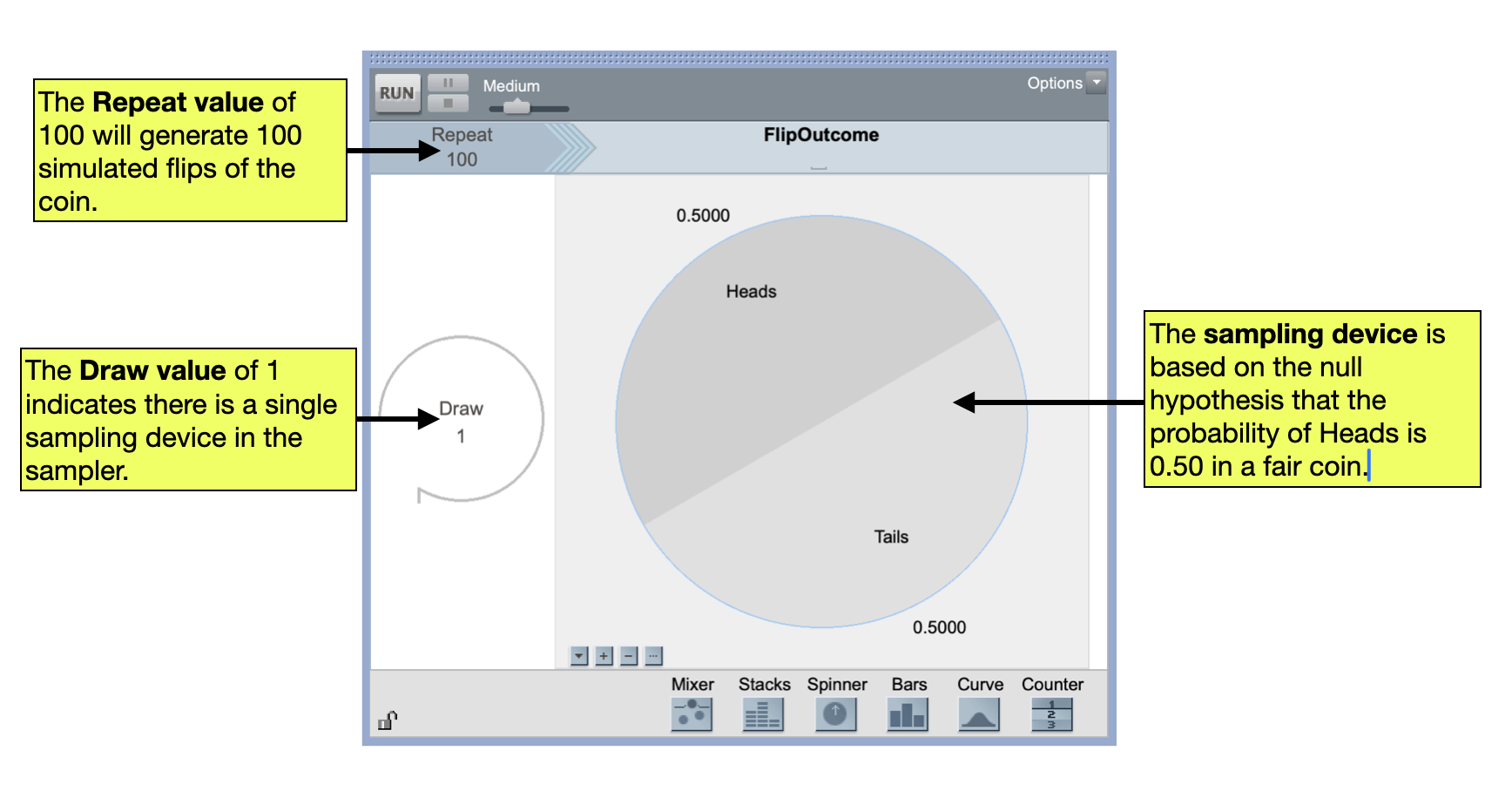
We can set up a TinkerPlots sampler based on this hypothesis. In our sampler, we need a device that has two potential outcomes (heads and tails). The heads outcome needs to have a probability of 0.50. We then set the repeat value to 100 to mimic our sample observed data in which we flipped the coin 100 times.
Simulate
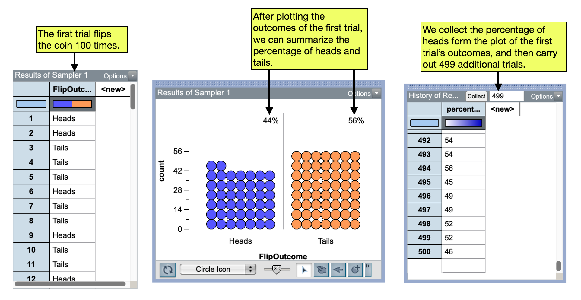
We can now use the model to produce the proportion of heads we would expect if we flipped the coin 100 times. To do this, we will run the simulation to obtain the outcomes from our first trial (i.e., 100 flips). After plotting those outcomes and summarizing them with the percentage of heads and tails, we could collect the percentage of heads. Then using the collect function, we could carry out an additional 499 trials (500 total trials).
Evaluate
To evaluate the hypotheses, we plot the summary measures from our 500 trials of the siumulation. This allows us to understand the sampling variation we expect if the null hypothesis is true.
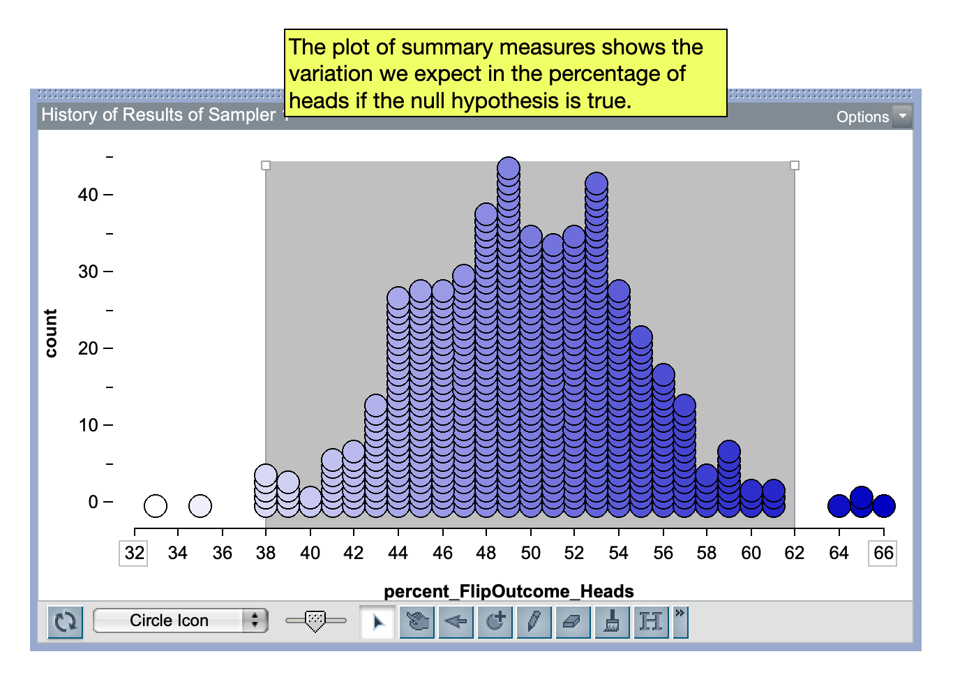
We can then use this plot to make a statement about which summary values we expect to see because of this sampling variation. In our example that might be the following:
If the null hypothesis is true, in 100 flips of a coin we expect to see between 38% and 62% of the flips to be heads.
That is, if we see that between 38% and 62% of the 100 flips to be heads it is consistent with the coin being fair. But, what we observed was that 64% of the 100 flips were heads. This is a higher proportion of heads than we expect if the coin were fair. Because our observed result of 64% heads was more extreme than what we expect if the null hypothesis is true, it acts as evidence against the null hypothsis. Because of this we would reject the null hypothesis that the coin is fair and conclude that the coin is indeed producing a higher percentage of heads than it should even after we account for the sampling variation.
In general Greek letters represent population parameters while Roman letters represent sample statistics.↩︎