TinkerPlots 101: Estimating Uncertainty via Bootstrapping
To illustrate how to compute compatibility intervals using TinkerPlots, consider the following example: A recent survey of randomly selected Australian teenagers asked about mobile-phone ownership. The survey was administered to 189 teenagers between the ages of 12 and 14. Results indicated that 138 of them owned a mobile-phone. The goal is to estimate the percentage of ALL Australian teenagers between the ages of 12 and 14 who own a mobile phone.
Point Estimate
Based on the observed data, our point estimate for the the percentage of all Australian teenagers between the ages of 12 and 14 who own a mobile phone is 73% (\(\frac{138}{189} = 0.73\)).
Margin of Error
When we use sample data to make a statistical estimate about the population, we need to incorporate the uncertainty due to sampling error into our point estimate. To do this we need to compute the margin of error, which is a measurement of the uncertainty in the point estimate. It turns out that we compute the margin of error similar to how we computed our range of likely values when we were testing hypotheses, namely:
\[ \mathrm{Margin~of~Error} = 2 \times \mathrm{Standard~Error} \]
That means, to compute the margin of error we first need to compute the standard error.
Bootstrapping
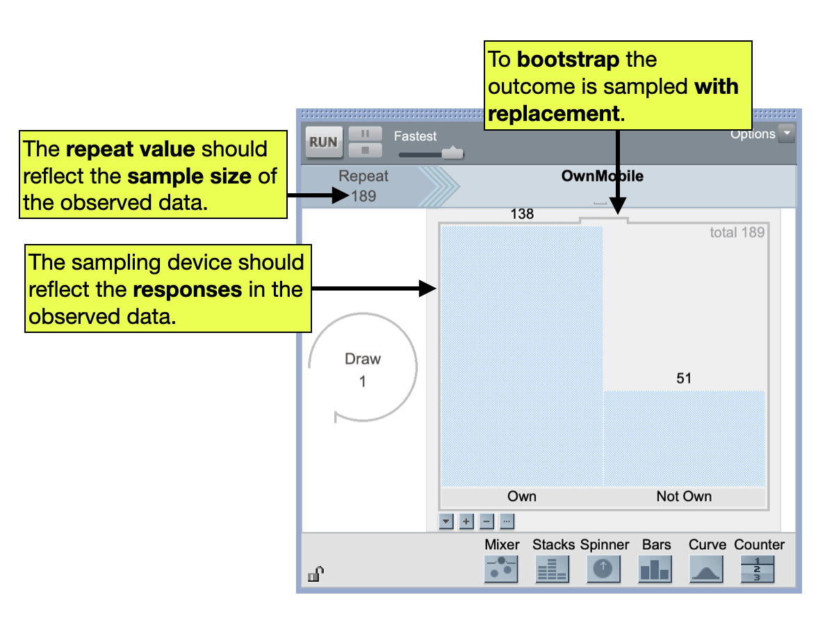
To compute the standard error in order to ultimately compute our margin of error, we will use TinkerPlots to model the sampling variation using the observed data. That is, we will set up a TinkerPlots sampler to bootstrap the observed data and collect the percentage of teenagers who own a mobile phone. Then we can compute the standard error of the bootstrapped results in the same way we have been in previous units. Figure 1 shows a TinkerPlots sampler to bootstrap from the observed mobile phone ownership data.
IMPORTANT
Because we do not have different groups of teenagers that we are comparing, we do not have a second sampling device to indicate groups like we did when we were comparing groups.
After running the first bootstrap trial, we can plot the simulated responses, and compute the percentage of teenagers who own a mobile phone. We can then collect an additional 499 percentages from this simulation. Figure 2 shows the distribution of the 500 bootstrapped percentages along with the computation of the standard error of these percentages.
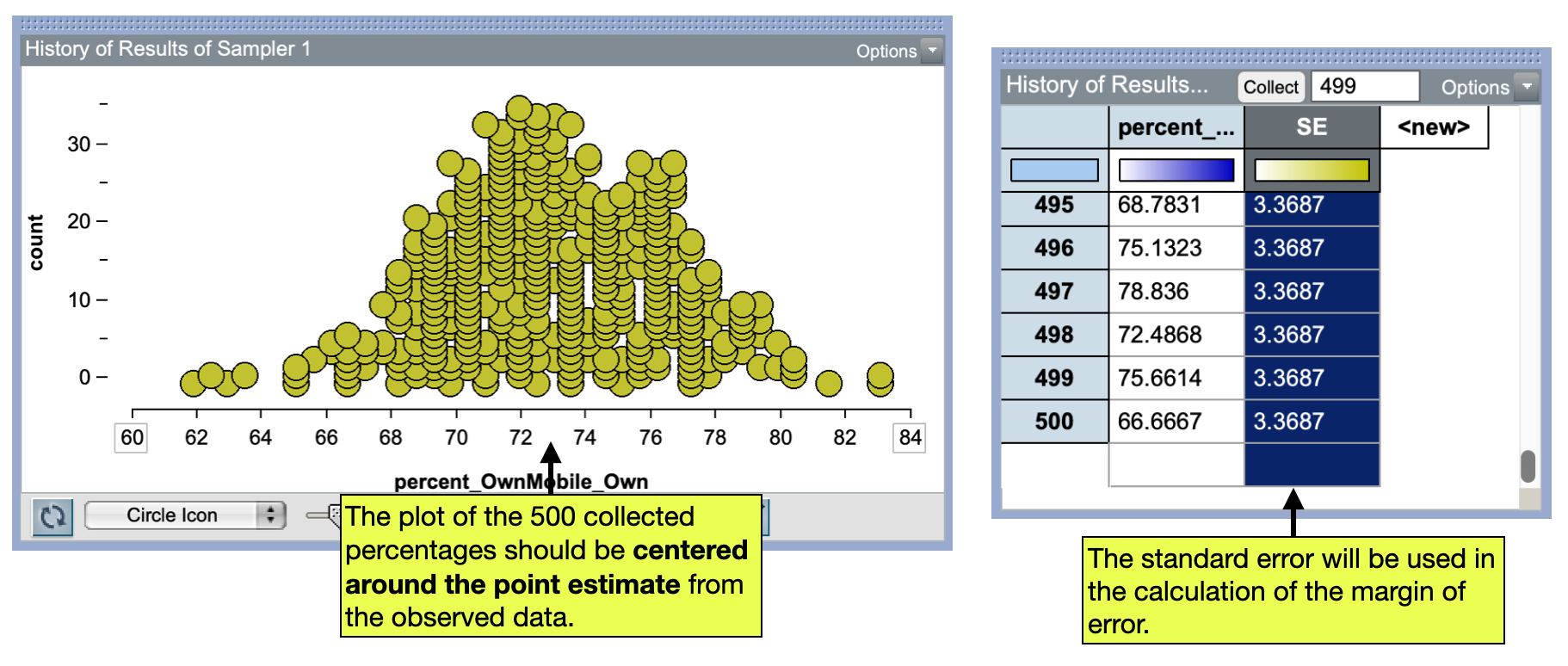
Because we are bootstrapping from the observed data (and not from a null model), the expected value is the point estimate from the observed data, namely 73%. (This is a check-in for you to be sure that the simulation was correctly set up; if the distribution of collected summary measures is not centered around the point estimate from the observed data—you did not set up the sampler correctly!)
The more important characteristic is to compute the standard error of the 500 bootstrapped percentages. We compute this the same as we always have, using the formula editor and the stdDev() function. Here the standard error is 3.37. This is a quantification of the sampling variation in our estimate. We can use this value to compute the margin of error:
\[ \begin{split} \mathrm{Margin~of~Error} &= 2 \times \mathrm{Standard~Error} \\ &= 2 \times 3.37 \\ &= 6.74 \end{split} \]
The margin of error for our point estimate is 6.74%. Note that the standard error and margin of error are two different values. The margin of error is twice that of the standard error. Both the standard error and the margin of error measure the uncertainty due to sampling variation. But, similar to why we used twice the standard error in our computation of the range of likely values when we were hypothesis testing, we will always use twice the standard error (the margin of error) when we compute compatibility intervals. (Remember, this is based on the Empirical Rule!)
LEARN MORE
You can learn more about the margin of error in What is a Margin of Error?, a chapter included in a short pamphlet put together by the American Statistical Association’s Section on Survey Research.
Computing the Compatibility Interval
Once we have our point estimate (73%) and the margin of error (6.74%), we can put those together to compute the compatibility interval:
\[ \begin{split} \text{Compatibility Interval} &= \text{Point Estimate} \pm \text{Margin of Error}\\ &= 73\% \pm 6.74\% \\ &= \big[66.26\%, ~~79.74\%\big] \end{split} \]
Recall that a compatibility interval acknowledges the uncertainty in the estimate by giving a range of potential values for the estimate of the parameter. Interpreting our compatibility interval:
We believe that the percentage of Australian teenages between the ages of 12 and 14 who own a mobile phone is somewhere between 66.26% and 79.74%.
Remember that our margin of error is based on two standard errors, and the Empirical Rule stated that because the distribution of bootstrapped percentages is roughly normal that roughly 95% of the bootstrapped percentages are within two standard errors of the point estimate (the expected value). Because of this, some statisticians embed this idea into their interpretation:
We are 95% confident that the percentage of Australian teenages between the ages of 12 and 14 who own a mobile phone is somewhere between 66.26% and 79.74%.
The “95% confident” part of the interpretation simply reflects the idea that we are measuring the amopunt of uncertainty by subtracting and adding two standard errors to our point estimate.