Quantifying Variation: The Standard Deviation
Recall that the mean is a single number that can be used to summarize the data; it is a summary of the typical value in the data. Of course, not every observation in a distribution is at the typical value (in fact all of them might be different from the typical value). Thus, it is also useful to have a summary measure of how different the data tends to be from this typical value. This summary is what statisticians refer to as the standard deviation. This measure quantifies variability by determining how far data cases typically deviate from the mean value.
Example Data
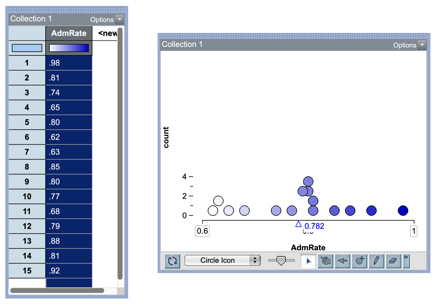
Consider the following data which give the admission rates for 15 public universities. The plot of the data suggests that the distribution of admission rates is unimodal and roughly symmetric. The mean admission rate for these universities is 0.782. There is also variability in the admission rates, with most univerisites in the sample having an admission rate between 0.7 and 0.9.
Calculating the Standard Deviation
The formula for the standard deviation is:
\[ \mathrm{SD} = \sqrt{\frac{\sum(x-\bar{x})^2}{n-1}} \]
while this may look ominous it really isn’t. The key is to break it down into its different steps.
- Calculate the deviations from the mean
- Square those deviations
- Sum the squared deviations
- Divide that sum by \(n-1\)
- Take the square root
Let’s walk through this with our admissions data!
Step 1: Calculate the deviations from the mean
Our first step is to calculate the deviations from the mean. To do this we take each data point and subtract the mean. For example, the deviation for the first admission rate is calculatedas:
\[ 0.98 - 0.782 = 0.198 \]
The positive value of the deviation tells us that this admission rate is higher than the mean admission rate by 0.198.
| Adm_Rate | Deviation |
|---|---|
| 0.98 | 0.198 |
| 0.81 | 0.028 |
| 0.74 | -0.042 |
| 0.65 | -0.132 |
| 0.80 | 0.018 |
| 0.62 | -0.162 |
| 0.63 | -0.152 |
| 0.85 | 0.068 |
| 0.80 | 0.018 |
| 0.77 | -0.012 |
| 0.68 | -0.102 |
| 0.79 | 0.008 |
| 0.88 | 0.098 |
| 0.81 | 0.028 |
| 0.92 | 0.138 |
Step 2: Square those deviations
In the next step we square the deviations we just calculated.
| Adm_Rate | Deviation | Squared.Deviation |
|---|---|---|
| 0.98 | 0.198 | 0.039204 |
| 0.81 | 0.028 | 0.000784 |
| 0.74 | -0.042 | 0.001764 |
| 0.65 | -0.132 | 0.017424 |
| 0.80 | 0.018 | 0.000324 |
| 0.62 | -0.162 | 0.026244 |
| 0.63 | -0.152 | 0.023104 |
| 0.85 | 0.068 | 0.004624 |
| 0.80 | 0.018 | 0.000324 |
| 0.77 | -0.012 | 0.000144 |
| 0.68 | -0.102 | 0.010404 |
| 0.79 | 0.008 | 0.000064 |
| 0.88 | 0.098 | 0.009604 |
| 0.81 | 0.028 | 0.000784 |
| 0.92 | 0.138 | 0.019044 |
Step 3: Sum the squared deviations
In Step 3, we sum all of the squared deviations.
\[ \begin{split} 0.15384 = 0.039204 &+ 0.000784 + 0.001764 + 0.017424 + 0.000324 + 0.026244 +\\ 0.023104 &+ 0.004624 + 0.000324 + 0.000144 + 0.010404 + 0.000064 +\\ 0.009604 &+ 0.000784 + 0.019044 \end{split} \]
Step 4: Divide that sum by \(n-1\)
In our sample we have 15 data points, so \(n = 15\). We are now dividing our sum of squared deviations by \(n-1\), or in our example, by 14.
\[ \frac{0.15384}{14} = 0.01098857 \]
Step 5: Take the square root
Finally we are going to take the square root.
\[
\sqrt{0.01098857} = 0.1048264
\]
Interpreting the Standard Deviation
To understand how we interpret this value, let’s again look back at the formula:
\[ \mathrm{SD} = \sqrt{\frac{\sum(x-\bar{x})^2}{n-1}} \]
Notice that the square root essentially removes the squaring that we did. If we omit the squaring and square root, that essentially leaves us with adding deviations and then essentially dividing by how many deviations there are. This is like the formula for average. So the standard deviation is essentially computing the average deviation from the mean. That is, it is indicating how far away from the mean value observations in the distribution are, on average.
In our example, the standard deviation was 0.1048. This tells us that, on average, the admission rates in our distribution are 0.1048 away from the mean. Another way to think about this is that most observations in the distribution are within 0.1048 units of the mean. Since the mean is 0.782, that tells us that most admission rates are in the range of \(0.782 \pm 0.1048\), or are between 0.6772 and 0.8868.
FYI
From statistical theory, we know that most of the observations in a distribution are within one standard deviation of the mean.
From the formula, we can also derive two other truths about the standard deviation.
- The standard deviation cannot be a negative value. While the deviations from the mean can be nagative, once we square these, they become positive. Also, remember that the standard deviation is measuring the average distance from the mean; distances are non-negative.
- The only way that the standard deviation ban be 0 is if every deviation is 0. That implies that every observation has the value of the mean. Another way to think about that is that every observation has to havethe same value—there is no variation.
Tinkerplots 101: Computing the Standard Deviation
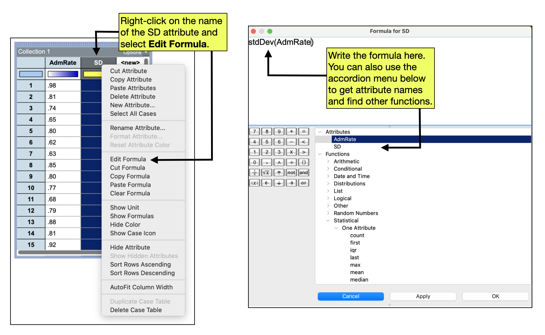
In practice, we will not use the formula to compute the standard deviation, but instead will use TinkerPlots to do the computation. Unlike other summary measures that we have computed (which are computed in the plot), the standard deviation is computed in the case table. To compute the standard deviation for the data in a case table, we first create a new attribute called “SD” in our case table.
- Click on the attribute name
<New>and edit the text toSD - Right-click the
SD(attribute name) and selectEdit Formula
This will open the formula editor. In the formula editor window type stdDev() which is the TinkerPlots formula for standard deviation. Inside the parentheses, we need to include the exact name of the attribute that you want to compute the standard deviation for. In our example, the name of that attribute is AdmRate. So the entire formula would read: stdDev(AdmRate).
- After you have entered your formula click the
Applybutton. This should populate theSDattribute in the case table with the value of the standard deviation. - Click
OKto close the formula editor.
Standard Deviation and the Normal Distribution
Earlier, it was pointed out that most of the observations in a distribution are within one standard deviation of the mean. For specific distributions we can be much more specific about the percantage of observations that are within one standard deviation of the mean. One of those distributions is the normal distribution. In the normal disribution 68% of the observations are within one standard deviation of the mean. We also know that 95% of the observations in a normal distribution are within two standard deviations of the mean, and 99% of the observations are within three standard deviations of the mean.
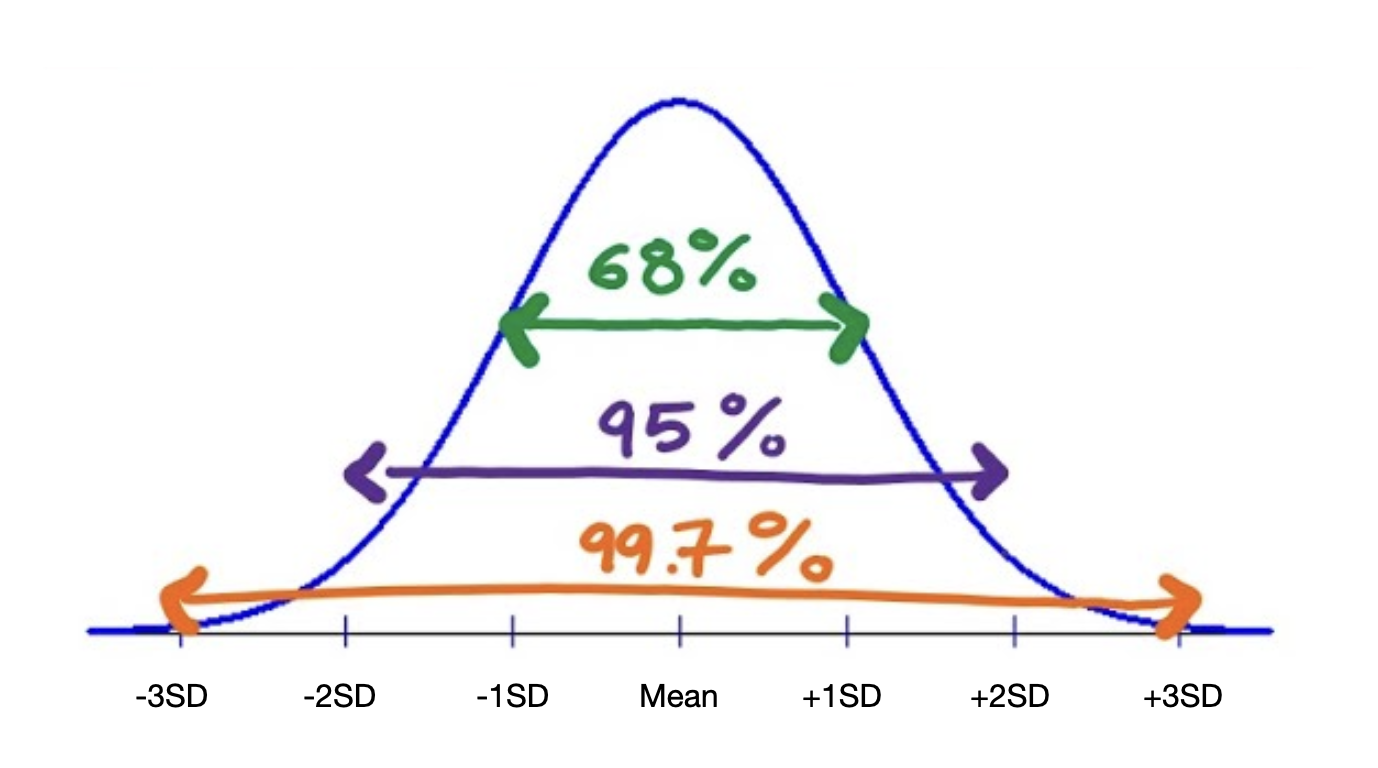
FWIW
This distribution of observations in the normal distribution is referred to as the Empirical Rule, or the 68–95–99 Rule.