Range of Likely Values
Recall that to evaluate a hypothesis, we build a model under the assumption that the null hypothesis is true, and then use that model to generate data from which we produce summary measures. We then create a range of likely values for those summary measures that we use to evaluate the summary measure from the actual observed data. Up until now, you have been eyeballing the distribution of summary measures and creating that range of likely values subjectively. We are now going to introduce a more formal method for creating that range of likely values. To formally create the range of likely values, we need two pieces of information:
- The expected value of the summary measure if the null hypothesis is true; and
- The standard error of summary measures.
To help us understand this, we will use the coin flip example introduced in Simulation Process for Evaluating Hypotheses. In that example, recall that we were evaluating whether or not the coin was fair, and the statistical hypotheses were:
\[ \begin{split} H_0:~ &\text{The proportion of heads when flipping the coin is equal to 0.50.}\\ H_A:~ &\text{The proportion of heads when flipping the coin is greater than 0.50.} \end{split} \]
Expected Value
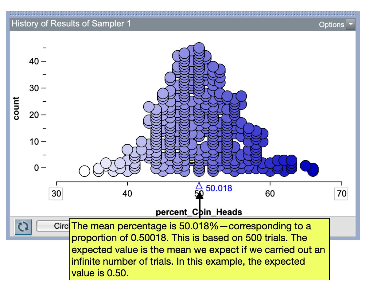
The expected value is the value for the summary measure that we expect under the null hypothesis. In our example, if the null hypothesis is true, we expect the proportion of heads to be 0.50.
\[ \text{Expected Value} = 0.50 \]
The expected value is a theoretical concept in that it is the mean value of the summary measure if we carried out the simulation an infinite number of times. If we look at the distribution of the proportion of heads in our 500 trials, you will notice that the mean is close to 0.50.
PROTIP
The mean of the collected summary measures in your simulation should be close to the expected value from the null hypothesis. If it isn’t, you may want to check that you carried out the simulation correctly. One common issue is that you collected the wrong summary measure (e.g., counts rather than percents).
Standard Error
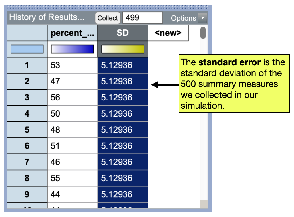
The standard error is a measure of the sampling variation we expect in a summary measure—a quantification of how much variation we would get simply because the summary measure is from a different sample. In practice, the standard error is the standard deviation we compute from the collection of summary measures in our simulation. In our example,
\[ \text{Standard Error} = 5.13\% \]
Or as a proportion,
\[ \text{Standard Error} = .0513 \]
Range of Likely Values
To compute our range of likely values we are going to combine the expected value and the standard error. Most statisticians define likely results as those that are within two standard errors of the expected value. (This is based on the Empirical Rule which states that in a normal distribution about 95% of the potential summary measures would be within two standard errors of the expected value.) The formula for the range of likely values is thus:
\[ \text{Range of Likely Values} = \text{Expected Value} \pm 2(\text{Standard Error}) \]
In our example, the range of likely values (for percent) would be:
\[ \begin{split} 50\% &\pm 2(5.13\%) \\ 50\% &\pm10.26\% \\ 39.74&\% \text{ to } 60.26\% \end{split} \]
Or, the range of likely values (for proportion) would be:
\[ \begin{split} 0.50 &\pm 2(0.0513) \\ 0.50 &\pm0.1026 \\ 0.3974& \text{ to } 0.6026 \end{split} \]
We can then use this to complete our sentence about what we expect under the null hypothesis:
If the null hypothesis is true (the coin is fair), out of 100 flips we expect to see a proportion of heads between 0.3974 and 0.6026.
We can then evaluate the actual observed data based on this range. Recall that we observed that 0.64 of the flips were heads in the actual data. This is outside the range of likely values—we observed a higher proportion of heads than we expect if the coin is fair. Because of this, we reject the null hypothesis which suggests that the coin may not be fair.